Report: LPSC 17002
MURE v.3 : SMURE,
Serpent-MCNP Utility for Reactor Evolution
User Guide - 2nd Edition
![]()
January 2024
Main Contributors :
-
O. Méplan (alias PTO), LPSC Grenoble
-
M. Ernoult (alias Xman), IPN Orsay
-
Maarten Becker (alias kernie), iUS Institut für Umwelttechnologien und Strahlenschutz, GmbH (Germany)
-
Jan Hajnrych, Ecole des Mines de Nantes, and Warsaw University of Technology (Poland)
-
A. Bidaud (alias le bid), LPSC Grenoble
-
S. David (alias GTS), IPN Orsay
-
X. Doligez (alias DodoXav), IPN Orsay
-
N. Capellan (alias Nico la Star), LPSC Grenoble
-
A. Nuttin (alias Nut), LPSC Grenoble
-
Frantisek Havluj, UJV, Czech Republic
-
Radim Vocka, UJV, Czech Republic
-
and in the past:
-
B. Leniau (alias BLG), Subatech Nantes
-
J. Wilson (alias JW), IPN Orsay
-
R. Chambon (alias Le caribou), LPSC, Grenoble, now back to Canada
-
F. Michel-Sendis (alias FMS), IPN Orsay, Now @NEA
-
F. Perdu (alias WEC), LPSC, Grenoble, Now @CEA
-
L. Perrot, IPN Orsay
-
Contents
- 1.1 Installation
- 1.1.1 Compilation
- 1.1.2 Remarks on MureGui compilation
- 1.1.3 Remarks on MCNP/makxsf compilation
- 1.1.4 Remarks on MURE with Serpent2
- 1.1.5 Building files for evolution
- 1.1.6 Running some examples
- 1.1.6.1 basic MURE possibilities
- 1.1.6.2 Fuel Evolution in a Sphere
- 1.2 MURE Package structure
- 1.3 MURE class
- 1.4 MURE basic files
3 From MURE to SMURE : Choosing the Monte-Carlo Transport Code
- 3.1 Switching from MCNP to Serpent in a MURE input file
- 3.1.1 Principle of the implementation
- 3.1.2 A example
- 3.2 How migrate my old MURE V1.x file to the MURE V2.x file
- 4.1 Introduction
- 4.2 Definition of geometrical shapes
- 4.2.1 Units
- 4.2.2 Examples of simple shapes
- 4.2.3 Examples of simple Nodes
- 4.2.4 Moving a Shape
- 4.3 The “put in” operator ">>"
- 4.4 Clone of a Shape
- 4.5 Boundary conditions
- 4.6 Recommendations
- 4.7 Definition of MC cells
- 4.7.1 Cell and clone shapes
- 4.8 Lattice
- 4.8.1 An implicit lattice example (SimpleLattice.cxx & SimpleLattice_serpent.cxx)
- 4.8.2 An explicit lattice example with different zones (SimpleLattice2.cxx & SimpleLattice2_serpent.cxx)
- 4.8.3 A lattice with more than one simple shape (Stadium.cxx & Stadium_serpent.cxx)
- 4.8.4 Lattice of a Lattice (LatticeOfLattice.cxx & LatticeOfLattice_serpent.cxx)
5 Materials, Sources, Tallies, ...
- 5.1 Definition of material
- 5.1.1 Clone
- 5.1.2 Mix (Mix.cxx)
- 5.1.3 Units
- 5.1.4 Material extension for MC
- 5.1.5 Pseudo Materials
- 5.1.6 MC material Printing
- 5.1.7 Examples
- 5.1.8 Automatic extension finding
- 5.1.9 Automatic XSDIR construction
- 5.2 Particle Source
- 5.3 Tally class
- 6.1 Nuclei Trees: general considerations
- 6.2 Nuclei Tree: the implementation
- 6.2.1 Important files
- 6.2.2 Reaction Auto-detection
- 6.2.3 The recursion depth cut
- 7.1 Preliminary Remark
- 7.2 General Considerations
- 7.2.1 Time discretization
- 7.2.2 The Bateman’s Equation
- 7.2.2.1 The evolution matrix
- 7.2.2.2 Multi-Threading parallelization
- 7.2.2.3 Cooling period
- 7.2.3 Solution of the Bateman equation
- 7.2.3.1 4th order Runge-Kutta
- 7.2.3.2 Chebyshev Rational Approximation Method (CRAM)
- 7.3 Different way of evolution
- 7.3.1 Cross-section Evolution
- 7.3.1.1 How does it work?
- 7.3.1 Cross-section Evolution
- 7.4 Reactivity Control
- 7.4.1 A simple example using standard EvolutionControl
- 7.4.1.1 Poison material declaration
- 7.4.1.2 Escape calculation
- 7.4.1.3 Evolution definition
- 7.4.2 Using your own EvolutionControl
- 7.4.1 A simple example using standard EvolutionControl
- 7.5 Evolution of a MCNP user defined geometry
- 7.6 More complex evolution conditions
- 7.7 Equilibrium of Xe-135
8 Looking at results from the evolution
- 8.1 The MURE data files
- 8.2 Reading the data files with Tcl/Tk graphical interface scripts
- 8.3 Reading the data files with ROOT graphical interface
- 8.4 Spectrum Classes (MCNP only)
- 8.4.1 Spectrum Class
- 8.4.2 GammaSpectrum class
- 8.4.3 AlphaSpectrum class
- 8.4.4 BetaSpectrum class
- 8.4.5 NeutronSpectrum class
- 8.4.5.1 Neutron from spontaneous fission
- 8.4.5.2 Neutron from (α,n) reactions
- 8.4.5.3 Neutron from (β−n) decays
- 8.4.6 Define MCNP Source with Spectrum object
9 Thermal-hydraulics/neutronics coupling
- 9.1 Preliminary Remarks
- 9.2 General Overview
- 9.3 Description of methods
- 9.3.1 Introduction
- 9.3.2 ReactorAssembly class
- 9.3.3 The COBRA_EN class : coupled neutronics/thermal-hydraulics calculations
- 9.3.3.1 Coupling Thermo-hydraulics and neutronics
- 9.3.3.2 Input/Output file
- 9.3.4 The BATH class (NOT YET TESTED IN SMURE-MURE v2.0)
- 9.3.4.1 Capabilities
- 9.3.4.2 What is solved
- 9.3.4.3 How to add data
- 9.3.4.4 Use the code
- 9.3.4.5 Output data
A Basic of C++ to understand MURE
- A.1 Introduction
- A.2 Class & Object
- A.3 Default arguments
- A.4 Pointers
- A.5 Inheritance
- A.6 Namespace
C Stochastic volume calculation
- C.1 Important Note
D Back-Stage processes: everything you always wanted to know about MURE* (*But were afraid to ask)
Chapter 1
Introduction
In the following, we refer either to MURE (MCNP Utility for Reactor Evolution), MURE ≥ 2 or SMURE (Serpent/MCNP Utility for Reactor Evolution)1 ; they represent the same package (MURE is the version 1 of SMURE-MURE ≥2). The main aim of the MURE[1, 2]/SMURE package is to perform nuclear reactor time-evolution using the widely-used particle transport code MCNP[3] (a Monte Carlo code which is mostly written in FORTRAN) or Serpent2[4, 5]. Many depletion codes exist for determining time-dependent fuel composition and reaction rates. These codes are either based on solving Boltzman equation using deterministic methods or based on Monte-Carlo method for neutron transport. Among them, one has to cite MCNPX/CINDER 90[6], MONTEBURN[7], KENO/ORIGEN[8], MOCUP[9], MCB[10], VESTA/MORET[11, 12], TRIPOLI-4D[13], Serpent[4], ... which provide neutron transport and depletion capabilities. However, the way to control (or interact with) the evolution are either limited to specific procedure and/or difficult to implement.
In (S)MURE, due to the Object-oriented programming, any user can define his own way to interact with evolution. From an academic point of view, it is also good to have lots of M-C evolution codes to compare and benchmark them to understand physics approximations of each one. Moreover, SMURE provides a simple graphical interface to visualize the results. It also provides a way to couple the neutronics (with or without fuel burn-up) and thermohydraulics using either an open source simple code developed in SMURE (BATH, Basic Approach of Thermal Hydraulics) or a sub-channel 3D code, COBRA-EN[14, 15]. But SMURE can also be used just as an interface to MCNP or Serpent to build geometries (e.g. for neutronics experiments simulation).
SMURE is based on C++ objects allowing a great flexibility in the use2. There are 4 main parts in this library:
-
Definition of the geometry, materials, neutron source, tallies, ...
-
Construction of the nuclear tree, the network of links between neighbouring nuclei via radioactive decays and nuclear reactions.
-
Evolution of some materials, by solving the corresponding Bateman’s equations.
-
Thermal-hydraulics: it couples neutronics, thermal-hydraulics and, if needed, fuel evolution.
-
Part 1 can be used independently of the 2 others; it allows “easy” generation of Serpent/MCNP input files by providing a set of classes for describing complex geometries. The ability to make quick global changes to reactor component dimensions and the ability to create large lattices of similar components are two important features that can be implemented by the C++ interface. It should be noted that some knowledge of MCNP or Serpent is very useful in understanding the geometry generation philosophy.
-
Part 2 builds the specific nuclear tree from an initial material composition (list of nuclei). The tree of each “evolving”3 nucleus is created by following the links between neighbours via radioactive decay and/or reactions until a self-consistent set of linked nuclei is extracted. Nuclei with half-lives very much shorter than the evolution time steps, could be removed from the tree; mothers and daughters of these removed nuclei are re-linked in the correct way. Part 2 can also be used independently of the other two parts to process cross-sections for MCNP/Serpent at the desired temperature.
-
Part 3 simulates the evolution of the fuel within a given reactor over a time period of up to several years, by successive steps of Serpent/MCNP calculation and numerical integration of Bateman’s equations. Each time the MC code is called, the reactor fuel composition will change due to the fission/capture/decay process occurring inside. Changes in geometry, temperature, external feeding or extraction during the evolution can also be taken into account. Obviously this part is not independent of the 2 others4 (see figure 1.1).
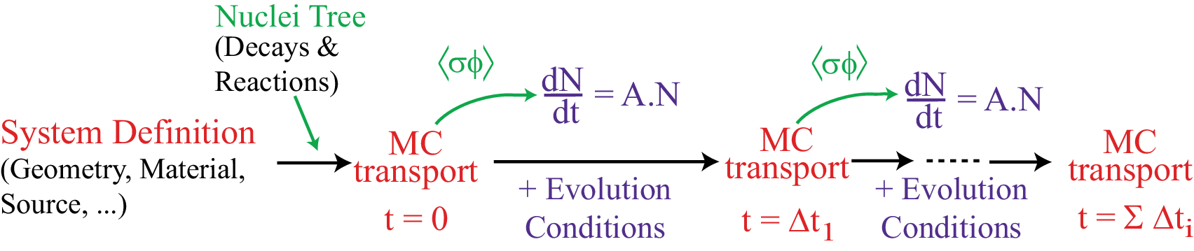
Figure 1.1: Principle of fuel evolution in MURE. -
Part 4 consists of coupling the Oak Ridge National Laboratory code COBRA-EN (COolant Boiling in Rod Arrays) with MURE. COBRA is a sub-channel code that allows steady-state and transient analysis of the coolant in rod arrays. The simulation of flow is based on a three or four partial differential equations : conservation of mass, energy and momentum vector for the water liquid/vapor mixture (optionally a fourth equation can be added which tracks the vapor mass separately). The heat transfer model is featured by a full boiling curve, comprising the basic heat transfer regimes : single phase forced convection, sub-cooled nucleate boiling, saturated nucleate boiling, transition and film boiling. Heat conduction in the fuel and the cladding is calculated using the balance equation.
The use of this package requires the following installation:
-
a C++ compiler (mandatory). SMURE is developed using gcc (for the more recent implementation the use of c++14 standard is required).
-
Serpent2, MCNP or MCNPX (mandatory, available at the NEA DataBank & RSICC). These codes will be referred as “MC” in the following.
-
Nuclear data files process for MCNP (ACE format) and/or NJOY[16] to process ENDF files into the ACE format (Nuclear data in ACE format are mandatory).
-
Serpent 1 can not be used with MURE because it does not support unions.
-
-
COBRA-EN for the thermal-hydraulic part (available the atNEA DataBank & RSICC)
-
The ROOT graphical tools developed at CERN (http://root.cern.ch) is necessary if user wants to use the post treatment GUI tools. In the GUI, radiotoxicity of fuel/waste can be calculated and plotted if the LAPACK library is installed (Linear Algebra PACKage, see http://www.netlib.org/lapack/index.html or standard LINUX repositories (Redhat, Fedora, Ubuntu, ...) for pre-installed versions). If you are using ROOT-5 or before, you should modify the beginning of the Makefile of MureGui.
At present, SMURE has only been compiled and tested on LINUX/UNIX platforms.
1.1 Installation
TO BE NOTICED: for some evident reasons5, upgrading for MURE version 1 to MURE version 2 breaks some backward compatibility. Nevertheless, for “old” MURE user changes will be minors ; we have try to keep the essential of MURE, but given more flexibility. A chapter is devoted to the migration of old MURE users.
1.1.1 Compilation
-
Uncompress the archive file where you want to install MURE source.
-
tar zxvf MURE_XX.tgz
or
-
gunzip MURE_XX.tgz ; tar xvf MURE_XX.tar
This will create the “data”, “documentation”, “examples”, “gui”, “lib”, “source” and “utils” directories in the MURE directory.
-
-
Configure and Compile MURE
-
cmake installation using “build.sh” script (Recommended)
-
in the MURE’s root directory, execute “./build.sh --enable-gui” will create everything needed for a default installation in MURE/mure3 directory (MCNP ≥5, with MureGui installed) using cmake. Default MURE install tree is
-
mure3/bin
-
mure3/include
-
mure3/lib
-
mure3/share which contains MURE data, examples, pdf and html documentation (user guide and class doxygen doc) in doc directory.
-
-
More options are available using this script : “./build.sh --help”
-
-
standard cmake installation
-
create a build directory in MURE root directory
-
cd build ; cmake .. for a default installation is for MCNP ≥5 and ENSDF in MURE directory.
-
or cmake [Arg] .. : where Arg could be
-
-DCUSTOM_INSTALL_PREFIX=path_to_install_dir (default=MURE root directory)
-
-DCMAKE_BUILD_TYPE=Release/Debug/RelWithDebInfo (default=Release)
-
-DUSE_OpenMP=ON/OFF (default=ON)
-
-DMCNPVersionNumber=4/5 (default=5 for MCNP version >= 5)
-
-DENSDF_path=path_to_ENSDF data (default="")
-
-DUSE_GUI=ON to build MureGui interface.
-
-
make [-jN] ; make install : compile on N threads & install MURE
-
-
-
Set shell’s environment variables (in your .bashrc or .tcshrc/.cshrc)
If you have used the build.sh script, the correct setting for (Linux) variables6 is proposed at the end of the script execution and it should look to something like that:
-
export MURE_DIR="/path_2_mure/MURE/mure3"
-
export MURECXXFLAG="-g -fPIC -std=c++17 -I$MURE_DIR/include"
-
export MURELIBFLAG="-L$MURE_DIR/lib -lMURE -lvalerr -lmctal -lnlohmann_json_schema_validator"
-
export PATH="${PATH}:${MURE_DIR}/bin"
-
export LD_LIBRARY_PATH="${LD_LIBRARY_PATH}:${MURE_DIR}/lib"
-
Remak:
-
The build.sh script defines the default MURE install directory as “MURE/mure3”. In the rest of this documentation, this directory is taken for sake of simplicity ; if you change it, replace this path by yours.
-
LD_LIBRARY_PATH is called SHLIB_PATH on HP-UX, LIBPATH on AIX or DYLD_LIBRARY_PATH on MacOS)
-
If during the “make” part of the install, there is an unsatisfied library dependence, you should install the “devel” version of this library (e.g. on FEDORA, ROOT-6 package relies on “liburing”, you should install “liburing-devel” package (via “dnf install liburing-devel”).
1.1.2 Remarks on MureGui compilation
The compilation is enable if you invoke “build.sh” script with “--enable-gui” or if you are using directly the “cmake” command, you should use the -DUSE-GUI=ON” flag.. Using MureGui without argument gives a short description of the code used (see also § 8.3). You need a modern version of ROOT (ROOT 5 or later). Optional libraries for radiotoxicity (LAPACK & BLAS) are also needed (in general, you need to install the “lapack-devel” on most of Linux distributions) ; installation of ROOT and these libraries are needed BEFORE running the “build.sh” script or cmake (or you have to re-run it).
1.1.3 Remarks on MCNP/makxsf compilation
In MURE, the access to ACE MCNP cross-sections is done for different purposes (find if cross-sections exist, find the total cross-sections in order to write in MC input file only “significant nucleus” (see 5.1.6), use of “multi-group flux” evolution method (see item 5 of section 7.3), ...). The use of binary ACE files improves the reading time (and also the disk space necessary to store the cross-sections). In C/C++, reading/writing in unformatted files (binary) is done by reading records of 1 byte long. But some FORTRAN compilers such as IFORT of Intel read/write in unformatted file with 4 bytes records. Thus if you want to use such a compiler for MCNP/makxsf you have to force the record length in unformatted files to be 1 byte. In the Intel IFORT compiler this is done via the –assume byterecl flag of ifort command line (see the System.gcf file of the config dir of MCNP distribution where System is either Linux, AIX, …).
1.1.4 Remarks on MURE with Serpent2
At the present time, Serpent2 seems only to handle ASCII file for ACE cross-section. Thus one has to use this ASCII data if one use Serpent. Conversion from the MCNP xsdir to Serpent xsdata is done either with the code provided with Serpent, either directly in MURE if one use the MURE:SetAutoXSDIR() method.
1.1.5 Building files for evolution
In this section, it is explained how to build the 2 necessary files BaseSummary.dat and AvailableReactionChart.dat (these files are not provided in the distribution). One supposes that a user has a standard MCNP6 ENDF B6 base provided with MCNP6. The provided xsdir file and the nuclear data are located in /path_2_ace_files directory (Verify that in the xsdir the absolute path to data files is present).
-
Then go to MURE/source/utils/datadir.
-
Compile the ExtractXsdir.cxx file (compilation line is at the end of the file).
-
Then run it with “ExtractXsdir”
-
Answer ENDFB to the first question
-
6.8 to the second one
-
/path_2_ace_files/xsdir to the third one
-
and STD to the last one.
-
-
After a while the BaseSummary.dat is created and contains the following
-
1 1 0 ENDFB 6.1 293.62 .24c STD 1001.24c 0.999170 /path_2_ace_files/la150n2 0 2 1 10106 4096 512 2.5301E-08
...
1 1 0 ENDFB 6.1 293.62 .66c STD 1001.66c 0.999170 /path_2_ace_files/endf66a2 0 2 1 10128 4096 512 2.5301E-08
...
92 235 0 ENDFB 6.1 293.62 .66c STD 92235.66c 233.025000 /path_2_ace_files/endf66c2 0 2 6899 722105 4096 512 2.5301E-08 ptable
...
-
Then compile (compilation line at the end of the file) and run CheckReaction
-
copy AvailableReactionChart.dat and BaseSummary.dat in MURE/mure3/data
-
Now you can run any examples of MURE.
1.1.6 Running some examples
The directory MURE/examples contains commented examples on how to use MURE. When this is possible, the same example exist for both MCNP and Serpent2; as it will be emphasis in the following, the differences in these 2 examples is generally limited to 3 or 4 lines to change, whatever the complexity of the system. A README file suggests an order to execute examples. For each example, a compilation line is put at the end of the file ; this line is based on the following environment variable definitions as defined in section 1.1.1 ; theses variables should be set in your bashrc (or cshrc, ...).
Here, 2 examples are described ; other examples are described in this User Guide (see for example, § 4.8.1, 4.8.2, 4.8.3 and 4.5).
In MURE/mure3/share/examples directory, one finds static examples (i.e. without burn-up calculations) and their outputs7 (in MURE/examples/Static/Reference_Outputs/ directory). To run some of these examples you must provide an MCNP xsdir file, whereas for other ones user has to build the BaseSummary.dat and AvailableReactionChart.dat files. The “evolution” examples are in MURE/mure3/share/examples/Depletion/ directory. Again you will find an “Reference_Outputs” directory that contains directory output of the examples (also gzip). In these result directories, one has suppressed the MCNP “o” and “m” files but left the MCNP input files as well as the MURE results files.
1.1.6.1 basic MURE possibilities
This example (MURE/mure3/share/examples/Static/Putin_example.cxx and MURE/mure3/share/examples/Static/Putin_example_serpent.cxx) shows basic geometrical methods.
-
The 2nd and 3rd line of these files says that the resulting files will be either MCNP or Serpent input.
-
Then a Connector plugin is built ; this connector links MURE object with Serpent or MCNP ones. It is MANDATORY.
-
One first builds 2 Materials (Graphite & Fuel).
-
Then pure geometrical Shapes are defined: in this example, one uses only Sphere.
-
The “put in” operator (">>") is used to put 3 spheres like Russian dolls: Smallest and Small are called Inside Shapes of Medium.
-
Then, this Medium “matrioshka” is duplicated with the Shape::Clone() method: the Medium2 clone is an exact copy of Medium: it contains a small sphere which contains a smaller one.
-
Medium and Medium2 shapes are then translated (with their inside shapes) and then put in the Big sphere.
-
Then, Cells are built (Serpent/MCNP cells): it associates a Shape with a Material. The exterior (outBig cell) is void and one has to specify a zero neutron importance because neutrons will not be followed (default importance is 1). For Serpent, this will correspond to the “outside” material. One has to build all Cells for all Shapes:
-
for Medium, Small and Smallest shapes, it is easy because they have been explicitly declared
-
Medium2 being a clone of Medium, it has also 2 inside shapes: thus one has to define cells for these inside shapes: one access to Shape::GetOriginalInsideShape() ; by convention, the most inner inside shape has the index 0, then the next one has the index 1, and so on.
-
-
And finally, the Serpent/MCNP file is built ; name is “minp” for MCNP input file and “sinp” for Serpent input file.
1.1.6.2 Fuel Evolution in a Sphere
The aim of this example8 of evolution (MURE/examples/Depletion/EvolvingSphere.cxx and MURE/examples/Depletion/EvolvingSphere_serpent.cxx) is to show basic burn-up calculation in MURE. The example describes a 50cm radius sphere with a inner sphere (R=30cm) of metal uranium, a middle ring (thickness=10cm) of UOx fuel and an external water reflector (thickness=10cm). The water will not evolve with time ; the thermal power of this “reactor” is 100 MW and it is kept constant for the whole evolution performed from t = 0 to t = 3 years.
-
After defining the Connector9, the file begins with some general MURE settings: DATADIR, Temperature precision, Fission Product selection, ...
-
Then 3 Materials are built: the water will not evolve whereas the metal and oxide uranium are evolving Materials.
-
Then Shapes are defined (the 3 spheres and the exterior of the “reactor”).
-
The Cell part associates Shapes and Materials.
-
Then one defines an isotropic, mono-energetic neutron source (500 n/batch) to run in critical mode (KCODE) with 30 active cycles, 10 inactive cycles and an estimated initial keff = 1.
-
The directory for the evolution is set (where MC files and evolution results will be written).
-
One important function concerning reactor evolution is to be called here : it is the thermal power at which evolution is to be simulated. This value is set using the gMURE->SetPower() where the argument must be in watts. (c.f. Steady-state Power Normalization in § D.1).
NOTE: For other applications or if the user already knows which neutron flux he wants to simulate, no power needs to be entered here but a tally normalization factor must then be specified. This Tally Normalization Factor can be set directly through the gMURE->SetTallyNormalizationFactor() method. -
Then one defines the 6 time steps at which a MC run is done, in a vector. The first MC step is always at time t=0 ; if this step is not defined, it will be insert in the vector. The evolution is performed up to the end but the last MC run is just the antepenultimate time step. This is important to know because this means the last values for keff, fluxes, cross-sections are not MCNP values: for keff the last value considered is the antepenultimate one.
1.2 MURE Package structure
The distribution package contains:
-
The PDF version of this user guide.
-
A complete useful description of each class (Doxygen headers documentation ; also available at the top of the html version of this guide)
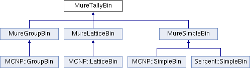
The general structure of main MURE’s classes is shown in figure 1.2.
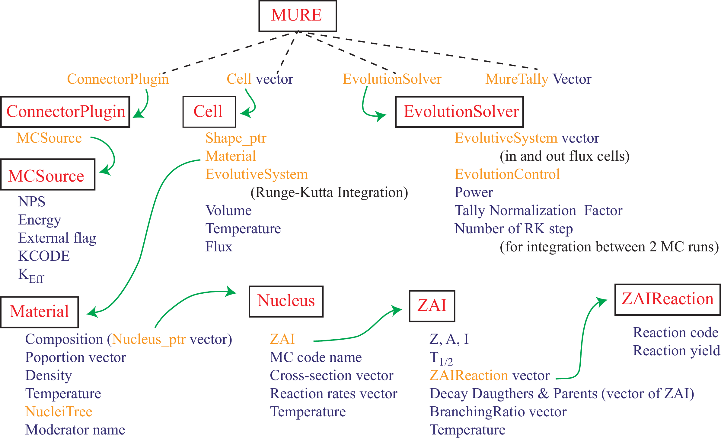
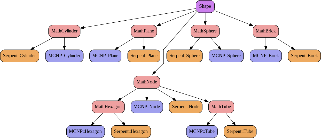
As it can be seen in figure 1.2, the link between classes is assured by the main class MURE. The Shape_ptr and Nucleus_ptr of the figure are smart pointer on Shape and Nucleus objects. The figure 1.3 shows the Shape inheritance graph using the 2 name spaces associated to the MC transport code used (MCNP or Serpent).
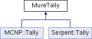
These name spaces are very important (see §3.1) ; one must use 1 (and only one) of them in any MURE input file. Results from MC run (Serpent detectors or MCNP tallies) are stored in the MureTally class which contains MureBin (cell, surface, ... bins) and TallyMultiplicator for reaction rates (see fig. 1.4 and 1.5).
1.3 MURE class
The MURE class is some kind of super class that handles connections between all the other classes. It controls all flows: MC input file writing, nuclei trees building, evolution, ...
A global pointer (gMURE) on this class is defined to allow interaction between classes. For example, when the geometry has been defined, as well as the MC source, tallies (or detectors), ...., the MC file will be written using
-
gMURE->BuildMCFile("myfile");
this will generate an MC input file called “myfile” (if no argument is given to the previous method, the default input file name is “inp”).
The name of MC exec command is given by
-
gMURE->SetMCExec("mcnp");
orgMURE->SetMCExec("sss2");
By default, MCNP::Connector set the the default value for the MC executable to “mcnp6” and Serpent::Connector set it to “sss2”.
MCNP Only: You can specify the particle running mode by either gMURE->SetModeN() (the default) to run MCNP with neutron transport, gMURE->SetModeNP() to transport neutrons and photons and so on. This is not take into account in the Serpent version.
Many methods exist and are grouped in sections to help the users ; therefore examination of MURE class header is strongly recommended (see Doxygen class description).
1.4 MURE basic files
Different files are used or built in MURE. It is important to know what these files are to understand the behavior of MURE.
1.4.1 Files of “MURE/mure3/doc”
This directory contains the most updated user guide and class documentations.
-
the “MURE/mure3/share/doc/pdf ” directory contains the PDF files
-
the “MURE/mure3/share/doc/html” directory contains the HTML files, in particular an HTML version of the user guide (which is a translation of the PDF one). HTML links are easier to use as well as copy/paste for examples. Moreover the “MURE/mure3/share/doc/html/doxygen” directory contains the automatic Doxygen description of classes.
1.4.2 Files in “MURE/data”
In the root MURE tree, there is a very important directory called “data” ; this directory is copied by the buid.sh script to MURE/mure3/share/data (known in MURE as the DATADIR) ; this directory can be set or changed by using either the environment variable DATADIR
-
export DATADIR=”$MURE_DIR/share/data”
or using the MURE::SetDATADIR() method10. In this directory, you will find:
-
chart.JEF3T: this (old) file contains, for each nucleus, the half-life time and the decay modes. It is a “hand-made” file from nuclear data book and JEFF 2.0 library, from "Nuclides and Isotopes", [17] and "Table of Isotopes", [18].
-
chart.jeff3.1.1: this file contains, for each nucleus, the half-life time and the decay modes. It is the updated version of the previous one and is the default. Data are extracted from NUBASE-2003, ENSDF, LNHB, UKHEDD-2.x and UKADD-6.x (see [19]).
-
Mass.dat and NaturalIsotopeMass.dat contain respectively the atomic mass for all nuclei and some natural compositions.
-
FPavailable.dat and FPyield.bin are fission product yield files: the first one is an ASCII file containing the Z,A of fissiles, and the address of the fission yield (for the available energies) in the binary FPyield.bin file. These files are built from ENDF/B-6.8 library. It is also provided FPavailable.dat.xx and FPyield.bin.xx where xx is either B6.8, B7.111 and J4_sep17 which are the files for ENDF/B-6.8, ENDF/B-7.1, and JENDL-4 (version of September 2017) which can be used. Source programs that build these files are in MURE/source/utils/fp. These files are part of the MURE package and have been built for 64 bits computers ; if you want to use other FP yield, you need to rebuild these files using MURE/source/utils/fp/GenerateFPYield.cxx (the compilation line is at the end of the file).
-
xsdirprequ.dat is the “header” of a general xsdir (from the top to the “directory” keyword). It is used in the automatic XSDIR construction for MCNP.
-
BaseSummary.dat is the file that contains all available nuclei, their temperature and the corresponding xsdir line.
It is build from MURE/source/utils/datadir/ExtractTree.cxx and/or MURE/source/utils/datadir/ExtractXsdir.cxx. The first one extracts information from a directory tree and the second from an existing xsdir. This file is the only way for MURE to use automatic MC nucleus code. The xsdata file for Serpent is also built from this file, using a conversion technique close to the perl script of Serpent. -
AvailableReactionChart.dat contains, for all nuclei of the chart.jeff3.1.1 (or the old chart.JEF3T) and BaseSummary.dat, whether or not reactions are available for MC codes. The aim of this file is to speed up the NucleiTree construction. It is built from MURE/source/utils/datadir/CheckReaction.cxx.
-
IsomerProduction.dat contains necessary information to allow the (n,γ) isomer productions for some important nuclei such as 241Am, 109Ag, …
NOTE: When you add new nucleus or temperature in nuclear cross-sections files, these modifications will be taken into account ONLY if BaseSummary.dat and AvailableReactionChart.dat have been updated. You also need to remove the local ReactionList directory (see after § 1.4.7).
1.4.3 Files of “MURE/source/utils”
This directory contains codes that can be very helpful to users.
-
“endf2ace” directory contains a small interface to NJOY (see documentation in the directory)
-
“fp” contains a utility to rebuild FPyield.bin and FPavailable.dat of MURE/mure3/share/data directory. Main file is GenerateFPYield.cxx which extracts from an ASCII ENDF file (containing the FP yields) the fission product yield in a format used by MURE.
-
“datadir” contains programs that allows users to build or complete the BaseSummary.dat and AvailableReactionChart.dat.
-
ExtractXsdir.cxx allows users to build/complete a BaseSummary.dat from an existing MCNP xsdir.
-
ExtractTree.cxx allows users to build/complete a BaseSummary.dat from a directory tree of cross-sections ; this tree can be built by the “endf2ace” utility. The form of the directory tree is
-
base_name/base_version/Z/AAA/Isomeric_state/temperature/bin/
where, for example, base_name=ENDFB, base_version=6.8, Z=92, AAA=235, Isomeric_state=0 (for ground state), temperature=600 (in K). In the directory “bin” one find the binary cross-section of the desired nucleus in the file “ace” and an xsdir line for this nucleus in a file named “dir” (for example the line looks like ’92235.10c 233.025000 ace 0 2 1 621851 4096 512 5.1704E-08 ptable’)
-
In both cases, the compilation line is at the end of the source code.
NOTE: If an existing BaseSummary.dat is already present in MURE/source/utils/datadir, this file is completed ; otherwise it is created.
-
CheckReaction.cxx must be used after building/modifying the BaseSummary.dat file in order to build the AvailableReactionChart.dat.
NOTE: After running ExtractXsdir/ExtractTree and CheckReaction, you have to copy the BaseSummary.dat and AvailableReactionChart.dat in your MURE/data.
-
1.4.4 Graphical User Interface “MURE/source/gui”
The GUI of MURE is located in the MURE/source/gui directory. The executable name is “MureGui” in the MURE/mure3/bin directory (if you ask for it in the installation procedure) and it reads the result of a MURE or Dragon evolution. To use it, user must install ROOT (free download at https://root.cern.ch). If the Lapack package is needed, (see http://www.netlib.org/lapack/index.htmll)12. Using MureGui without argument gives a short description of the code used (see also § 8.3 ).
1.4.5 “MURE/source/external” and “MURE/source/thirdparty”
-
MURE/source/external contains libraries developed before MURE project that are useful to deal with MCNP output file reading (mctal library) as well as handling value and error of a number (ValErr library).
-
MURE/source/thirdparty contains
-
The Eigen library[20] ; this library is used for CRAM (see §7.2.3 integration. It is automatically downloaded and install with build.sh/cmake install.
-
The JSON library[21, 22] ; this library is used for the result of evolution data in the ASCII JSON format. It is automatically downloaded and install with build.sh/cmake install.
-
1.4.6 MURE Source files
The MURE source files are located in “MURE/source/include” for the header files (.hxx) and in “MURE/source/src” for implementation (.cxx). When user is modifying the MURE source, he has to recompile the MURE package (by a “build.sh” script or cmake13). In MURE/source/external, one finds 2 auxiliary libraries, ValErr and Mctal that are used in MURE. The ValErr defines a class to handle numbers and their errors, and Mctal is dedicated to reading/writing MCNP “m” files.
In any program using MURE, you have to include at least:
-
#include >MureHeaders.hxx>
and either one of the following
-
#include <MureMCNPHeaders.hxx>
or
-
#include <MureSerpentHeaders.hxx>
If needed on can add also :
-
#include <libmctal/TMTally.hxx>
#include <libmctal/TMComment.hxx>
#include <libmctal/TMctal.hxx>
1.4.7 Other files
Each time a new evolution is run, a directory ReactionList is locally built (if it is not already there) with the available reaction of user’s nuclear data base (one binary file for each Z). A list of suppressed reactions for some of the nuclei (because they are lower than a given threshold) is also written in ReactionList/SuppressReaction.dat. The aim of theses files is to save time when using the same nuclear data base AND the same reaction threshold, life-time cutting and so on. Thus if you modify one of these, DO NOT FORGET to remove the ReactionList directory.
Chapter 2
What’s new in MURE
-
January 2024:
-
add a MureConsole, a kind of “text” version of MureGui to extract as text data from a single evolution directory ; The Console class, called by MureConsole, should be modified to extract your particular data ; it provided an example which should by easy to modify for your own purpose. The compilation is down via make -f Makefile.console.
-
Modify the GenerateFPYield (version 2) to be able to generate FP independent yields from different ENDF libraries where data are provided as a single file or in multiple files ; all the files of the provided directory will be used as ENDF file format to extract FP yields for MURE evolution. A ReadFPyield code can be used to extract a given FP yield distribution as a function of the mass.
-
-
December 2021: MURE/SMURE Version 3!
-
Use smart pointer for gMURE and gTREE : each ZAI is now unique and only provided by the gTREE smart pointer.
-
Evolution data can be written (when ASCII is chosen) with the JSON format via the EvolutionSolver::SetWriteJsonFormat().
-
Complete MURE directory tree reorganization:
-
the root MURE tree contains: cmake, data, doc, examples, source ans tests directories as well as CMakeLists.txt and build.sh (for cmake install), LICENSE and README.md file.
-
source directory contains: src, include, utils, gui and external
-
the new install procedure is based on cmake (using either direct cmake command or the recommended build.sh install script)
-
and the default install directory is now mure3 (in MURE root directory) with a share dircetory (containing a copy of examples, data and doc (pdf, html)), include, lib and bin (with MureGui) ; this evolution allows a clear separation between MURE sources and user’s files.
-
change environment variables setting to take theses changes into account (see build.sh script for correct setting)
-
-
Modernization of the code (all source code) according to c++11 standard.
-
Many small (or not) bugs have been corrected (in particular in ReactorAssembly) and a great effort has been done in fixing memory leaks (rewrite of many constructors and destructors, used of smart pointers)
-
documentation update.
-
-
February 2021
-
rewrite examples tree structure
-
update doc (lyx & html & User Guide & doxygen)
-
change compilation line in examples: it is now based on 3 environment variables (that should be defined in your bashrc or cshrc or ...) :
-
export MURE_DIR="/path_2_MURE_install_dir/"
export MURECXXFLAG="-g -fPIC -std=c++14 -I$MURE_DIR/source/include -I$MURE_DIR/source/external \
-I$MURE_DIR/source/thirdparty/eigen"
export MURELIBFLAG="-L$MURE_DIR/lib -lMURE -lvalerr -lmctal"
-
-
January 2021
-
Implementation of the CRAM (Chebyshev Rational Approximation Method) method to solve Bateman equations (which is the new default to solve Bateman equation). This new implementation has been done by Maarten Becker.
This implies some changes in method names and reorganization of Evolution related classes :-
RK discretization is now called sub-steps discretization and EvolutionControl methods using “RK” use now “SubStep”.
-
Two new classes, CRAMSolver and RKSolver have been created and the depletion method is chosen by either
-
gMURE->GetEvolutionSolver()->SetDepletionSolver("RungeKutta")
or
gMURE->GetEvolutionSolver()->SetDepletionSolver("CRAM").The latter is the default. These classes inherit from BatemanSolver and the previous DynamicalSystem class is removed.
-
-
A new Timer class has been added to store time spent (to replace OMP omp_get_wtime(), ...).
-
The compilation of SMURE require at least “c++11” standard.
-
MureGui update: try to read DATA_* files if BDATA_* files are not found (avoid the use of “-type A”).
-
The MURE library has been rename libMUREpkg.so as libMURE.so : you must change the linked library name in your project
-
a cmake installation is now available (see paragraph 1.1.1)
-
remove 32 bit systems support
-
-
February 2019
-
Add a new button in MureGui (Inventory Tab) to plot inventories in atom percent of the total of selected nuclei ; this allows for example to obtain the plutonium vector at any time of an evolution.
-
-
November 2016:
-
Add Z revolution axis Torus for MCNP and Serpent ; see MathZTorus , MCNPZTorus and SerpentZTorus classes.
-
Update “chart.jef3T” file that contains periods and decay modes for all the chart ; this file (JEFF 2 lib.) is kept unchanged, but a new file has been created “chart.jeff3.1.1” (from ref. [19]); it is the new default.
-
-
November 2015:
-
ReactorMesh and ReactorChannel class have been removed ; a new GenericReactorAssembly, and its concrete versions MCNP::ReactorAssembly and Serpent::ReactorAssembly replace the ReactorMesh class. It is a complete rewriting of that class, bu the spirit is kept (see § 9.1 and 9.3.2). It adds lot of new possibilities (add duct to an assembly, filling core with a ReactorAssembly, ...).
-
COBRA class is renamed COBRA_EN and rewritten ; again backward compatibility is broken (it does not inherit from GenericReactorAssembly) but the spirit is not changed.
-
-
October 2015:
-
Correct a bug when reading the “standard” xsdir of MCNP5 ; isomeric cross-section libraries are now in accordance with the MCNP5 documentation.
-
-
July 2015:
-
New MURE version 2.0 (SMURE). This is a major release of MURE. It couples now both MCNP & Serpent. Due to technical, philosophical difficulty and also to beauty in programming (dry codes), backward compatibility is broken. But the changes to user input files between MURE v1 and MURE v2 are small. See 3.
-
-
November 2014:
-
Add the possibility to use standard MCNP tallies 238U and multi-group tallies for other nuclei (see 5).
-
-
October 2014:
-
Add an optional equilibrium treatment for 135Xe (see 7.7)
-
-
April 2013:
-
Version of base and isomeric states (metastable and ground state) for 242Am in BaseSummary.dat file for standard library (distributed with MCNP or available@NEA) are now more conform to the reality ; you have to regenerate your BaseSummary.dat/AvailableReaction.dat files with the exec of MURE/utils/datadir. DON’T FORGET TO REMOVE YOUR ReactionList DIRECTORY IN ORDER TO TAKE INTO ACCOUNT THESE MODIFICATION.
-
BasePriority has been debug and it seems to work as expected...
-
-
March 2013:
-
Add a generalization of the MURE::SetMode() method to allow any type of particle transport (mainly for MCNPX)
-
Cell importance may have different value for each transported particles (by successive call to Cell::AddParticle method)
-
extend the MCNPSource possibilities (particle distributions are now allowed for MCNPX)
-
-
July 2012:
-
Generalization of isomer production by (n,γ) for special cases (such as 241Am, 109Ag, …), and bug correction in (242Cm, 242Pu) production, see 6.1.6.
-
Improve MurGui Spectrum radiotoxicity tab
-
Allow to plot neutron balance in the “Reaction Rate” tab.
-
-
June 2012:
-
Add functions in MureGui (see MureGui’s Radiotoxicity tab)
-
Nuclei extraction is now possible after a given cooling time.
-
γ,β, α and neutron spectra for evolving materials can be computed.
-
-
New MURE install procedure (more simple, more robust): any fresh install or update NEED to run first the install.sh script (require bash shell).
-
Add the possibility to used multi-threading (OpenMP) during the evolution and for updating multigroup σϕ when the gcc version support this option (see INSTALL procedure and install.sh script and section 7.2.2.2).
-
Add some new kind of MCNPSource (see section 5.2.3)
-
Add fluence to dose conversion for tallies
-
-
May 2011:
-
Add a new class GammaSpectrum class (section 8.4.2)
-
New option of MureGui : use the “radiotoxicity tab” of MureGui on a dumped Material created with MURE (see 8.3.6 and “MURE/example/GammaSpectrumExample.cxx”)
-
New methods MCNPSource::SetAXS and MCNPSource::SetVec allows user to define collimated sources.
-
In Tally::Tally(int type,const char *particle) : if type < 0 , it’s change the Tally units.
-
For example Tally *t=new Tally(-4,"P") define a tally in MeV∕cm2 rather than Particles∕cm2 .
-
-
A new method MURE::SetModeP() can be used to allow only the photon transport.
-
-
July 2009:
-
Improve the English in User Guide: many thanks to Erica Agostinho for this painful work.
-
Implementation of PseudoMaterial: in order to take into account temperature effects, one can process the nuclear data at the desired temperature (using NJOY ) or use an interpolation between 2 already existing temperatures ; this later method is used in the PseudoMaterial techniques.
-
-
Avril 2009: MURE is available at NEA DataBank
-
January 2009:
-
Improve reading time of BaseSummary.dat file : it is now greatly recommended that this file is ordered by Z,A,I (this is the case if it is generated by ExtractedXsdir.cxx and ExtractTree.cxx).
-
Rewrite long parts of the documentation (User Guide and HTML class description)
-
Modify examples directory: it now contains documented examples and output.
-
-
November 2008: Improve radiotoxicity post treatment in MureGui.
-
September 2008: Implement “multigroup” calculation for reaction rates: a very narrow energy binning for flux calculation is put in each MCNP run ; then reaction rates are obtained by reading ACE MCNP files after each MCNP run. The result of such method saves a considerable amount of CPU time for MCNP (at least a factor 30) with only a low percentage of discrepancy (∼1 to 3%) in result compared to the standard calculation (reaction rates are tallied in MCNP).
-
April 2008:
-
implementation of Predictor-Corrector method in the evolution
-
possibility to read ASCII nuclear data file (ACE format): this avoids problems due to binary compatibility (size of real (float or double?), little or big endian, ...). BUT it is much longer to (1) build the ReactionList directory and (2) run a MCNP.
-
-
December 2007:
-
Disable the σϕ extrapolation by default. It has been shown, but not really understood, that this treatment introduces a larger dispersion in the result, after N identical evolutions, than doing nothing (no σϕ extrapolation).
-
Modify the evolution using a MCNP User Input geometry file:
-
“like but” cells can be used (but not evolved)
-
“MCNP Transformation” cards can be used
-
the 3rd block of the MCNP file is read and copied except the materials (that must be defined in the MURE file). Thus the source as well as all other cards of this block can be used without defining them in the MURE file (this is also true for user defined tallies).
-
-
-
October 2007:
-
Switch from ccdoc to Doxygen for class documentation
-
Change completely the MURE directory trees
-
NON BACKWARD COMPATIBILITY
-
Material definition has changed: now only 2 constructors must be used:
-
Material(): for standard material (you have to specify density, ... with the Set methods)
-
Material(int): for using materials from an MCNP input file geometry.
-
-
THE COPY CONSTRUCTOR HAS NOT TO BE CALL: CALL only the Material::Copy().
-
The Material::Mix has been modified (number of arguments, units required). see Material.hxx
-
The Material::AddNucleus has been modified (number of arguments). By default the proportion units are "kpMOL" (i.e. molar proportion). But the unit must be specified if you use a moderator (MT card of MCNP).
-
The proportion units (both for Density and Proportion) must be used for any Material::GetProportion() and Material::GetDensity() methods
-
for Proportion the only valid units are: kpMOL(molar prop), kpMASS (mass prop), kpATCM3 (at/cm3), kpATBCM(at/barn.cm)
-
for density the only valid units are: kdGCM3 (g/cm3), kdATCM3 (at/cm3), kdATBCM (at/barn.cm)
-
-
A new material has been defined : ControlMaterial (public of Material). This class is used for Poison, Fissile or other control of reactivity (e.g. poison.cxx in MURE/examples)
-
All Print() methods now return a string instead of a void: to use them: cout<<Mat->Print()<<endl; for example.
-
EvolutionControl class has been cleaned (as well as MURE class). If you want to use special control you have to write your own derivative class. Examples using PoisonControl, FissileControl & HNControl (but Adrien you have to rewrite them and look carefully at TMSR.cxx in MURE/examples.) and Rod control are defined in source/src. You can used them as they are or defined your own using these examples.
-
-
Almost all cout/cerr have been removed from classes; used instead LOG_DEBUG, LOG_INFO, ... ; LOG_INFO is now independent of LogLevelMessage ; it is always printed. If MURE::SetMessageLevel is set to LOG_LEVEL_DEBUG, all LOG_DEBUG are printed. But if MURE::SetSilentDebug is used, only the LOG_DEBUGs of methods where a "int DODEBUG=1" is inserted are printed. Thus, using LOG_DEBUG, avoids to comment all "cout" when no debugging is desired.
-
ALL EXAMPLES HAVE BEEN UPDATED TO TAKE INTO ACCOUNT THESE MODIFICATIONS: please READ THEM!!!!!!!!!!
-
-
September 2007:
-
Correct an important bug in evolution using an MCNP User Input geometry file: number of Materials were not correct (Thanks to Jan Frybort).
-
-
Juin 2007:
-
Rename the MURE header file Shapes.hxx into MureHeaders.hxx : this is more logical...but you have to change your MURE files....
-
Add a new class EvolutionWrapper to simplify and extend EvolutionControl capabilities
-
Suppress the writing of BDATA_xxx and DATA_xxx ; now, by default, only BDATA_xxx are written. This can be changed using the MURE::SetWriteBinaryData() and MURE::SetWriteASCIIData() methods.
-
One can start an evolution from a given step : suppose that the evolution stops at step i ; an evolution can be started from the step i+1 using MURE::Evolution(T,i+1). Warning: it is probably not correct for OutCoreEvolutiveSystemVector...you must do the evolution from the first step as before.
-
Chapter 3
From MURE to SMURE : Choosing the Monte-Carlo Transport Code
As already said, coupling MURE with a other MC code had 2 consequences:
-
decouple MURE from MCNP, which was a big job because they were closely linked.
-
couple MURE to a MC code (Serpent or MCNP), which is also a big job because the Serpent an MCNP philosophy are sometimes completely different.
The aim is with a minor change to input file, it will be able to generate output for MCNP or for Serpent 2. In this chapter, it is explained first how to switch from an MCNP input file to a Serpent input file (or vice-versa) and then how to migrate from MURE 1.0 to SMURE (MURE 2.0) .
3.1 Switching from MCNP to Serpent in a MURE input file
SMURE has been designed to make the change from Serpent input to MCNP input (or vice-versa) as simple as possible. Of course, Serpent is not MCNP and conversely. Thus each of these MC codes have their own possibility, not implemented in the other. Moreover, the maturity of the MURE coupling is much greater (few years of work for MCNP versus 4 months of work for Serpent). Thus this section deals only with things that are possible with both MC codes and has been implemented in MURE. Nevertheless, it seems to us that is it enough to make a standard reactor study (including evolution).
3.1.1 Principle of the implementation
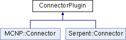
In MURE, the choice of MC output is performed via a ConnectorPlugin ; this class has 2 sibling, a MCNP::Connector and a Serpent::Connector (see Fig. 3.1) ;
thus the main trick is the use of a specific namespace (MCNP or Serpent). Geometrical shapes are defined in MURE as MathShape (i.e. a “pure” mathematical Shape, e.g. a MathSphere). Then, in each namespace, are defined concrete (or real) shapes that essentially provide a print method derivating from the MathShapes (see Fig. 1.3). For example, a Serpent::Sphere and MCNP::Sphere are daughters of MathSphere and implement a Serpent::Sphere::Print() or a MCNP::Sphere::Print() that will produce respectively the right output for the corresponding MC code. The same trick applies for tallies (or detectors in Serpent).
Thus, using a Connector, a Sphere, ... in MURE is just “resolved” by the namespace (that should not be forgotten). In order it works without problems, appropriate header files must be included. First header file, is the “pure” MURE header : MureHeaders.hxx which includes all pure MURE classes. It is thus included in all MURE input files, whatever will be the output. The second header file is linked to the output ; MureMCNPHeaders.hxx and MureSerpentHeaders.hxx includes all classes that couple MURE with MCNP and Serpent respectively. They include particularly MCNP::Connector (Serpent::Connector), MCNP::Sphere (Serpent::Sphere), ...
Of course connectors, because of some profound differences between MCNP & Serpent, have specific methods existing only in one type of connector. The same applies also for the Tally class which is more complete in MCNP. The last case is for particle sources which are very different from MCNP to Serpent. This is why, sibling of MCSource class keep the MC code prefix in there name (MCNPSource and SerpentSource) in order that the user don’t forget its specificity. An other cause of problems, switching from one code to the other is the MURE::AddSpecialCard() which allows to use specific Serpent or MCNP cards that have not been implemented in MURE. Thus a careful check of Connector, MCSource and MURE::AddSpecialCard() should be done when switching from one code to the other.
3.1.2 A example
Switching from one MC code to the other can be performed very fast : edit the file (let say a MCNP version) and replace all “MCNP” string by “Serpent” string. This should change 4 occurrences: the header, the namespace and the source name (See example of Tab. 3.1). Then remove specific command for MCNP and add specific command for Serpent. To illustrate this, let us consider the “evolving sphere” example. The “red” parts of Table 3.1 correspond to a “replace all” “MCNP” string by “Serpent” string. The magenta words are “output” directory name, that here, are different to keep a trace of both evolution. The blue lines is an example of a pure specific method of one code (here MCNP) of one of the 3 classes Connector, (MCNP/Serpent)Source or Tally. And then, in green, a MURE::AddSpecialCard() that in this case is only for Serpent.
|
|
|
|
|
|
|
|
As Shown on this example, the number of line to modify is very limited ; moreover, dealing withe a more complex case, this number will not increase significantly (probably less than a factor 2).
3.2 How migrate my old MURE V1.x file to the MURE V2.x file
3.2.1 What has definitely change
In this part, only the coupling with MCNP is considered (as in the old MURE v1). Main changes are due to
-
Header file has change (row 1 of the Tab. 3.2) ; one must use a namespace MCNP.
-
One has to define a ConnectorPlugin of type MCNP::Connector (see row 1 of Tab. 3.2) just after the main declaration. The connector is responsible for all pure MCNP methods. Row 3 of Tab. 3.2 give an example for removing MCNP “r” files; but the same apply for SetPRDMP(), SetMCNP4B() which are now in MCNP::Connector and no more in MURE.
-
Method names of MURE containing “MCNP” are (in general) now named with “MC” ; examples are given from row 4 to 7.
-
Evolution is no more in MURE class but in the EvolutionSolver class ; example of change are given in row 8 to 10. Almost all MURE evolution related method are now in EvolutionSolver excepted MURE;SetPower() and MURE::Evolution().
-
Lattice implementation has changed :
-
Replace the declaration from a simple Cell to a LatticeCell (row 11)
-
the Cell::Lattice() is replaced by LatticeCell::SetLatticeRange() and the lattice type is no more necessary (see row 12)
-
-
ReactorChannel & ReactorMesh classes: the first one is, since a while, obsolete ; it is removed in MURE V2.0. The second one has been deeply rewritten and rename as ReactorAssembly but the spirit has not change ; most of work (and thus time spent to migrate from MURE V1.x to MURE V2.0 will be in the change of this ReactorMesh to ReactorAssembly class but we think that the improvements of ReactorAssembly justify this “extra-work”. For more details on the ReactorAssembly class see section 9.3.2.
|
|
|
|
MURE version 1 |
MURE version 2 : SMURE |
|
|
|
|
|
|
|
#include <MureHeaders.hxx> |
#include "MureHeaders.hxx" |
|
#include "MureMCNPHeaders.hxx" |
|
|
using namespace MCNP; |
|
|
|
|
|
int main(...) |
int main(...) |
|
{ |
{ |
|
Connector *plugin=new Connector(); |
|
|
gMURE->SetConnectorPlugin(plugin); |
|
|
|
|
|
gMURE->SetRemove_r_files(); |
plugin->SetRemove_r_files(); |
|
|
|
|
gMURE->BuildMCNPFile(); |
gMURE->BuildMCFile(); |
|
gMURE->SetMCNPInputFileName("inp"); |
MURE->SetMCInputFileName("inp"); |
|
gMURE->SetMCNPRunDirectory("sphere","keep"); |
gMURE->SetMCRunDirectory("sphere","keep"); |
|
gMURE->SetMCNPExec("mcnp5"); |
gMURE->SetMCExec("mcnp5"); |
|
|
|
|
gMURE->SetWriteASCIIData(); |
gMURE->GetEvolutionSolver()->SetWriteASCIIData(); |
|
|
|
|
gMURE->UseMultiGroupTallies(); |
gMURE->GetEvolutionSolver()->UseMultiGroupTallies(); |
|
|
|
|
gMURE->SetUseNewDBCN(); |
gMURE->SetUseNewRandomSeed(); |
|
|
|
|
Cell *MyLattice=new Cell(AGenerator); |
LatticeCell *MyLattice=new LatticeCell(AGenerator); |
|
MyLattice->Lattice(1,-rx,rx,-ry,ry,-rz,rz); |
MyLattice->SetLatticeRange(-rx,rx,-ry,ry,-rz,rz); |
|
} |
} |
|
|
|
The time spent to change a very big file from version 1 to version 2 is around 5 minutes maximum.
3.2.2 What is still existing but can be done in a more elegant way
In most of real case fro reactor physics, one has to use lattice, fuel pin, ... A new improvement of MURE version 2 is to implement a PinCell which in fact copy the elegant Serpent’s pin definition. To illustrate the advantage of such a PinCell class, the main part of the lattice example in the “old” way is presented and then rewrite using PinCell. For sake of clarity, only Shape and Cell part are presented. All sizes have been defined, as well as 3 Materials : H2O, Iron, and UOx. As shown on Tab. 3.3, the use of PinCell makes the code shorter (the 8 blue lines of the shape declaration have been suppressed), and easier to define and to read. The PinCell declaration make cell part slightly longer (4 ”magenta” lines versus 6 “green” lines). To be noticed, the use of a PinCell without a layer allows to define the whole universe. And a last comment on the FillLattice methods : in the first version, a Shape is used as argument (red variables on the left) where as in the new version this is a PinCell (red variables on the right).
|
|
|
|
|
|
|
|
Thus user is strongly encourage to use these PinCells.
Chapter 4
Geometry Definition
4.1 Introduction
C++ logic for building geometries is slightly different for the MCNP or Serpent one ; therefore, each time a new geometry is built you should check it with MCNP/Serpent before using it.
There are two base classes to build a geometry: Shape and Cell. Shape describes only geometrical shapes, and Cell corresponds to an MC code cell (i.e., it has a material, importance, etc.).
Shape objects correspond to simple geometrical shapes (sphere, plane, ...) as well as more complex ones resulting from the intersection and/or union of simple shapes (Intersections/unions are defined by the Node class). A Node is a “tree” of intersections/unions of Shapes. For fast calculations, a node tree has to be as simple as possible. Special methods are available for simplifying the node trees which can (in general) determine whether or not a Shape is disjointed (or included) of (in) another Shape (see example in figures B.1 to B.4 in Appendix A.6).
These simplifications may result in the deletion of some Shapes. But, because one must not destroy a Shape in a Node if that Shape belongs to another Node, a special way to handle Shape creation/destruction has been implemented (via Reference_ptr, which is a C++ smart pointer).
In conclusion : the user must only use Shape_ptr (a “reference Shape”) and not Shape. Shape_ptr is a pointer to Shape with Reference_ptr. In that way, the Shape_ptr will be destructed only if it is no longer referenced, otherwise, its “deletion” leads to a decrement of the number of references.
4.2 Definition of geometrical shapes
-
There are 4 available base Shapes :
-
Plane (infinite),
-
Cylinder (infinite),
-
Sphere,
-
Brick (finite or infinite)
-
-
Then one can define Node (unions or intersections of Shapes) with 2 already defined Nodes:
-
Tube
-
Hexagon (finite or infinite)
-
A Brick is a rectangular parallelepiped (and can be infinite). A Tube is a finite cylinder with an optional inner radius that defines a “tube”. Hexagons can have finite or infinite height. In general, a user will only need to use Spheres, Bricks, Tubes and Hexagons.
One can define the interior or the exterior of each Shape. The complement of a Shape can be defined by the Not() method as well as by the “!” operator (see examples given later on).
Other shapes available in MCNP(X) or Serpent may be added by any user. This is not too hard even if it requires some work. The best way to do it, is to read the implementation of existing shapes to have an idea.
4.2.1 Units
WARNING: In MURE, the length unit is the meter (whereas in MCNP and Serpent it is the cm). In particular, volumes in MURE are in m3.
|
|
|
| Length | m |
|
|
|
| Energy | eV |
|
|
|
| Temperature | K |
|
|
|
| Density | g/cm3, atom/cm3 or atom/(barn.cm) |
|
|
|
| Proportion | %mol, %mass, atom/cm3 or atom/(barn.cm) |
|
|
|
4.2.2 Examples of simple shapes
To define the interior of a origin center sphere of radius R:
-
Shape_ptr S(new Sphere(R));
To define the outer part of S one can do
-
Shape_ptr Ext_S(!S);
or
-
Shape_ptr Ext_S(S->Not());
or
-
Shape_ptr Ext_S(new Sphere(R,0,0,0,1);
where 3 zeros correspond to the sphere center (the origin) and +1 to the exterior of the Sphere (default=-1).
For Hexagons and Bricks, two versions exist: finite or infinite Shapes. For finite bricks and hexagons, you should define it as:
-
Shape_ptr B(new Brick(HalfX, HalfY, HalfZ, Signe));
Shape_ptr H(new Hexagon(HalfHeight, Side, Signe));
where HalfX (resp. Y and Z) is the Half length of the brick in the X (resp. Y and Z) direction, HalfHeight the half height (!) of the hexagon, Side its side, and Signe the sign defining whether it is the inner or the outer part, just as for the sphere. For infinite ones, to avoid conflicts between the definitions, a string at the beginning is necessary (and, of course, HalfHeight and HalfZ are irrelevant) :
-
Shape_ptr B(new Brick(“any string you want”, HalfX, HalfY, Signe));
Shape_ptr H(new Hexagon(“any string you want”, Side, Signe));
The infinite shapes obtained are parallel to the Z axis, but they may be rotated afterwards.
4.2.3 Examples of simple Nodes
A Node is the Union (+1) or the Intersection (-1) of Shapes (i.e., simple Shapes or Nodes).
To define the intersection of a sphere centered at (x0,y0,z0) of radius R with a square brick of side a centered at the origin, one may use:
-
Shape_ptr S(new Sphere(R,x0,y0,z0);
Shape_ptr B(new Brick(a/2,a/2,a/2));
Shape_ptr Inter=S & B;
whereas the union of the sphere and the brick may be defined as
-
Shape_ptr Union=S | B;
4.2.4 Moving a Shape
It is possible to move (translation/rotation) a Shape (or a Node) via the Shape::Translate and Shape::Rotate methods. For example, to translate the Shape_ptr B of (dx,dy,dz),
-
B->Translate(dx,dy,dz);
and to rotate clockwise B around (x0,y0,z0) of ϕ, 𝜃 and ψ around the z, y and x axis respectively:
-
double center[3]={x0,y0,z0};
B->Rotate(phi,theta,psi,center);
Note that the translation/rotation of a Shape translates/rotates also the inside shapes (see next section).
To be noticed: Angles are in radians.
4.3 The “put in” operator ">>"
It is possible to put a Shape_ptr A inside another B one, via the “put in”1 operator A>>B ; this operator works differently depending on A:
-
if A is a normal Shape_ptr: a A>>B modifies both A and B ; A becomes A ∩ B and B becomes B∩!A (see figure 4.1)
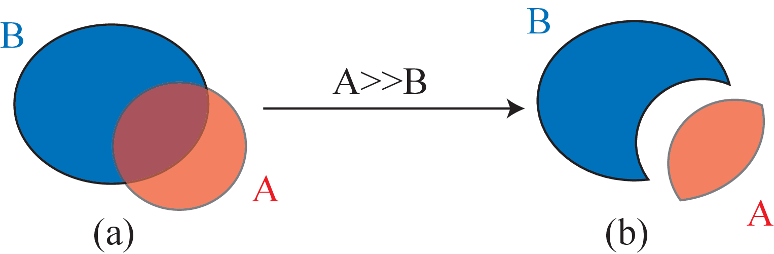
Figure 4.1: Operator >> (put in). (a) A and B before the action of the operator ; (b) A and B after the action of the operator. -
if A is a Shape_ptr with a universe number (e.g. after a call to Shape_ptr::SetUniverse() for a lattice): A>>B does not modify neither A nor B ; a MCNP Fill card is just added to B in order to fill B with universe of A.
Example:
-
Shape_ptr S(new Sphere(R));
Shape_ptr B(new Brick(a/2,a/2,a/2));
B>>S;
In this example, the Brick B is put inside S.
Note that now S and B are new Shape_ptr: S=S & !B (i.e. the sphere without the brick) and B=S & B (i.e, the intersection of the brick and the sphere) as already mentioned above (see fig. 4.1).
-
The brick B is an inside shape of S: this means that if one moves S, one moves also B.
-
It is possible to link inclusion:
-
A>>B>>C;
means that A is put in B and the result is also put in C. A is an inside shape of B and C ; B is an inside shape of C.
-
if after the previous example, one makes
-
C>>D;
Inside shapes of C are cleared and D has A, B and C as Inside Shapes.
4.4 Clone of a Shape
It may be sometimes very useful to clone a Shape, i.e., to create a new Shape with the same properties as the original one. Here is an example:
-
Shape_ptr B1(new Tube(1,0.5));
Shape_ptr T1(new Tube(1,0.4));
Shape_ptr T2(new Tube(1,0.3));
T2>>T1>>B1;
Shape_ptr B2=B1->Clone();
B2->Translate(1,0,0);
B2 has exactly the same aspect as B1 (with 2 tubes inside) but it is translated by 1m in the x direction, whereas B1 is centered at the origin.
4.5 Boundary conditions
In MCNP, it is possible to use special boundary conditions: mirror, white or periodic boundary conditions. In Serpent, boundary conditions can be applied only on the shapes associated to cells with the “outside” Serpent’s material. The only valid possibilities for Serpent are black (totally absorbing, the default), mirror or periodic.
To be noticed also, the “outside” cells of Serpent don’t support unions. For any geometry, if the outside cell (Serpent namespace only) is not a “simple” shape (simple in the Serpent’s sense, it includes Spheres, unrotated Tubes, Bricks or Hexagons), then the user define outside shape (the one which is in the 0 importance cell) is put into a Sphere.
In Serpent, boundary conditions only apply to Bricks (square, cuboid, ...) or Hexagons (hexxc, hexxprism, ...). Mirror and Black boundary conditions have been implemented in MURE for unrotated Bricks or Hexagons in Serpent. In any case, the use of boundary conditions in MURE could be used but have not been fully tested...so it is advised to use them carefully. In all cases, the exterior of the Shape_ptr with boundary conditions must have a zero importance. You can apply only one type of boundary conditions to a Shape_ptr. Here is a brief description of these boundary conditions:
-
Mirror conditions correspond to a standard reflection on a shape ; the method to define such conditions is
-
Shape_ptr A(...);
A->SetMirrorBoundary();
-
-
For some shapes, (Hexagons and Bricks) mix boundary conditions can be used (e.g. x-y surfaces are mirrors whereas top and bottom z-planes are open (black)).
-
White conditions correspond to a reflection with a cosine direction distribution on the surface ; the method to define such conditions is
-
Shape_ptr A(...);
A->SetWhiteBoundary();
-
-
Periodic condition: when a particle leaves a given plane it re-enters through another one. This method could only be applied to Bricks or Hexagons, with the restriction that the Top and Bottom planes (before any reflections) are either Mirror boundaries, White boundaries or Infinite boundaries.The method to define such conditions is
-
Shape_ptr A(new Brick(1,1,1));
A->SetPeriodicBoundary(true,"mirror");
or
-
Shape_ptr A(new Brick(1,1,1));
A->SetPeriodicBoundary(true,"white");
-
4.6 Recommendations
-
It is generally simpler to define a geometry from the inner part to the outer part : for example,
-
define first shape A, then B and C and D.
-
Put shapes inside each other like
-
A>>B>>D;
C>>D;
-
After doing that, you can’t move and/or rotate A, B or C. But if you move/rotate D, then it will move/rotate also the inner shapes (A, B and D). If A, B or C have to be rotated or translated to a given position in D, then you must do it BEFORE putting these shapes inside D.
-
-
Avoid complex shapes: it is more efficient (in term of CPU time at least for MCNP) to divide a complex in several simpler shapes.
4.7 Definition of MC cells
A Cell is defined by a Shape_ptr, and if needed a Material.
MC cells are defined via the Cell class ; one has to give
-
the Shape_ptr corresponding to the geometric shape of the Cell,
-
the Material (see section 5.1) if exists (default=0 for void),
-
the importance of particles2 (default=1),
For example to construct a cell composed of a full tube of radius R and height H, made of B4C
-
Shape_ptr C(new Tube(H/2,R));
Cell* c=new Cell(C,B4C);
where B4C is a (Material*)3. In this example, one can define the exterior cell as
-
Shape_ptr Exterior(!C);
Cell* exterior=new Cell(Exterior,0,0);
The first zero means that the material is void and the second one means that neutron importance is set to 0 in the exterior cell (“outside” material for Serpent).
NOTE: If not only neutrons are transported in MCNP, it is useful to define the desired mode (i.e., NP, NE, NPE for Neutron and Photon, Neutron and Electron and Neutron, Photon and Electron) before any Cell definition ; indeed, in this case, the given cell importance applies to all particle types. For example:
-
gMURE->SetModeNP();
Cell *c=new Cell(C,B4C);
Cell *exterior=new Cell(Exterior,0,0);
will set the transport mode to neutrons and photons and the cell c will have an IMP:N=1 and IMP:P=1 whereas the cell exterior will have an IMP:N=0 and IMP:P=0.
4.7.1 Cell and clone shapes
Suppose we have defined 2 tubes B1 and B2 as follows:
-
Shape_ptr B1(new Tube(1,0.5));
Shape_ptr T1(new Tube(1,0.4));
Shape_ptr T2(new Tube(1,0.3));
T2>>T1>>B1;
Shape_ptr B2=B1->Clone();
B2->Translate(1,0,0);
the cell definition for B1 is not a problem:
-
Cell *b1=new Cell(B1,Graphite);
Cell *t1=new Cell(T1,Iron);
Cell *t2=new Cell(T2);
where Graphite and Iron are two Material*. Here, the result will be a tube of graphite containing a tube of iron containing a void tube. To define analog cells for B2 we have to do:
-
Cell *b2=new Cell(B2,Graphite);
Cell *tt1=new Cell(B2->GetOriginalInsideShape(1),Iron);
Cell *tt2=new Cell(B2->GetOriginalInsideShape(0));
Indeed, the “Inside shapes” of B2 are ordered from the most inner (B2->GetOriginalInsideShape(0) clone of T2), to the most outer (B2->GetOriginalInsideShape(1) clone of T1).
4.8 Lattice
Lattices are used in MC to fill cells of repeated structure. In MCNP, there are 2 types of lattice, hexahedra (type=1) or hexagonal (type=2). In Serpent, circular lattice are also defined but they are yet not implemented in MURE.
In this section, four examples of lattices are presented (from the most simple to the most complex case). Of course the lattice type does not change the declaration (except that the lattice generator is a Brick for hexahedra lattice whereas it is an Hexagon for the the hexagonal one). Lattice philosophy is somehow different from MCNP and Serpent ; the MURE implementation is closer to the MCNP’s one.
The general philosophy for lattice declaration is the following:
-
In the Shape section
-
define the Shape_ptr C that will be filled by the lattice (like core),
-
define the Shape_ptr G that is used as lattice generator (a Brick or an Hexagon) and give to that generator a universe number (via Shape::SetUniverse()),
-
put G in C with G>>C
-
define all Shape_ptr Bi that shall be used in the lattice and assign them a universe number (via Shape::SetUniverse()) or use PinCell (see (a) of Cell Section)
-
-
In the Cell section
-
define PinCell Pi (and/or use (d) of previous part)
-
build the Cell for Shape_ptr C
-
build the LatticeCell with the generator Shape_ptr G
-
[optional] indicate to LatticeCell the extension of the lattice (via LatticeCell::SetLatticeRange() or LatticeCell::SetNumberOfLatticeElement())
-
fill the lattice with all the desired Shape_ptr Bi and/or the PinCell Pi (via LatticeCell::FillLattice())
-
4.8.1 An implicit lattice example (SimpleLattice.cxx & SimpleLattice_serpent.cxx)
This example illustrates implicit lattices, that is to say a lattice filled by a unique universe. A simple tube (a Vessel) is filled by an hexagonal lattice. Each hexagon of the lattice is made of water and filled with a small cylinder of UOx fuel (a pin) inside an Iron cladding. For this example, 2 different implementation are propose to illustrate the only use of shape (like in the 1.d of the beginning of this section) or the use of PinCell (like in 2.a ).
|
|
|
|
|
|
|
|
As it can be seen, the version using PinCell is more compact and more easy to understand (Blue part disappear and magenta part is replaced by green one ; the lattice is thus filled by the PinCell). These two implementations give the same result which is shown in Figure 4.2. Note that in the first implementation, outside of the cladding (OutClad Shape) has the same universe than the Clad Shape because it is define as the complementary Shape of Clad (the ! operator). Note also than OutClad and Exterior shapes must be defined before the “put-in” operator (>>) because this latter modify the definition of Vessel or Clad. Few words for Serpent users: the “lat” card of Serpent need an origin, and a pitch. These quantities are deduced from the generator shape ; translating it will thus change “lat” origin. The sizes of the generator shape will determine the pitch (number of values as well as values depending on the dimension (2D or 3D) of the lattice).

4.8.2 An explicit lattice example with different zones (SimpleLattice2.cxx & SimpleLattice2_serpent.cxx)
Explicit lattices are filled with different universes, allowing to put different structures at some given position. To illustrate this, let us modify the previous example slightly: we want to fill the Vessel with 2 types of hexagons: the first ones are full water hexagons (the reflector) in the outer part of the Vessel and the second ones are the previous hexagons with the small pin rod inside. For shortness, we chose to fill the Vessel with second hexagon type if it is inside a “virtual” cylinder of radius 90cm. Both implementations using Shape only or PinCell has been proposed in Tab. 3.3. Here, a focus is made on the PinCell implementation. The principal changes take place between the lines named “Line A” and “Line B” . We have to replace this part by:
-
//-------------------- Line A --------------------
PinCell* whole=new PinCell;
whole->SetSurroundingMaterial(H2O);
LatticeCell *Pavage=new LatticeCell(LatticeGenerator);
int range=int(VesselR/(1.5 * HexaSide))+1;
Pavage->SetLatticeRange(-range,range,-range,range); //define a explicit lattice
for(int i=-range; i<=range; i++)
for(int j=-range; j<=range; j++)
{
int pos[3]={i,j,0}; //the lattice index
double xt = HexaSide*sqrt(3.) * (i + j*0.5 ) ;
double yt = 1.5 * HexaSide * j;
double X[2]={xt,yt}; //the center of each hexagons
if(IsHexagonInTube(X,LatticeGenerator,0.9)) //true if the hexa center at X is
Pavage->FillLattice(pinUox,pos); //inside a tube of radius 90cm
else
Pavage->FillLattice(whole,pos); //inside a tube of radius 90cm
}
//-------------------- Line B --------------------
-
A new PinCell (whole) is defined ; because just a surrounding material is defined, this PinCell represents the whole space (it is a “pseudo-PinCell”).
-
Then the lattice range is defined as (2range+1)×(2range+1) matrix (in x and y direction and infinite in z). The “range” has been defined to cover at least the entire vessel.
-
Then, each position of hexagons in the lattice is computed ; if a hexagon is inside the virtual cylinder of radius 0.9m, a hexagon with the pin rod is used (PinCell pinUox in the Cell::FillLattice method) at the given position pos else the “whole” PinCell is used (and as always with lattices, it is automatically cut by the lattice meshes).
The result is shown in Figure 4.3.
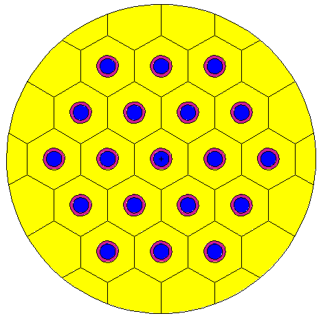
Note: if one prefers use only shapes (and not PinCell), one can used the following trick (but it is not implemented for Serpent!!!)
-
In the Shape part, define a Shape_ptr corresponding to the Whole space (intersection of nothing4):
-
Shape_ptr Whole(new Node(-1));//-1=intersection, here, of nothing
Whole->SetUniverse();
-
and in the Cell part, add
-
Cell *whole=new Cell(Whole,H2O);
-
4.8.3 A lattice with more than one simple shape (Stadium.cxx & Stadium_serpent.cxx)
In this example, we consider a hexahedra lattice. Each brick of the lattice will have parts of “stadiums” on each (x,y) sides (see Figure 4.4, this is the base geometry of the MSRE reactor).
-
//
//materials
//
Material *Salt=new Material(); //this is the fuel LiF-ThF4/UF4
Salt->SetDensity(3.1);
Salt->AddNucleus(3,7,0.7);
Salt->AddNucleus(9,19,1.9);
Salt->AddNucleus(90,232,0.15);
Salt->AddNucleus(92,233,0.15);
Material *Graphite=new Material();
Graphite->SetDensity(1.86);
Graphite->AddNucleus(6,0,1);
//
// Data
//
double VesselH=0.8; // the core H and R
double VesselR=0.4;
double SquareH=VesselH; //stadium heigth
double SquareS=0.2; //stadium straight line length
double BendR=0.02; //stadium bend curve radius
double BendH=VesselH;
double BrickW=0.04;
double BrickL=0.08;
//
//Shapes
//
//the Vessel
Shape_ptr Vessel(new Tube(VesselH/2,VesselR));
//the Exterior
Shape_ptr Exterior(!Vessel);
//the lattice generator
Shape_ptr LatticeGenerator(new Brick(SquareS/2,SquareS/2,SquareH/2));
LatticeGenerator->SetUniverse();
//put the lattice generator inside the core
LatticeGenerator>>Vessel;
//Definition of the stadiums (horizontal & vertical)
Shape_ptr Circle0(new Tube(BendH/2,BendR));
Circle0->SetUniverse();
//clone circles for horizontal and vertical stadiums
Shape_ptr Circle1=Circle0->Clone();
Shape_ptr Circle2=Circle0->Clone();
Shape_ptr Circle3=Circle0->Clone();
//translate circle
Circle0->Translate(-0.1,+0.04,0);
Circle1->Translate(-0.1,-0.04,0);
Circle2->Translate(-0.04,0.1,0);
Circle3->Translate(+0.04,0.1,0);
//2 bricks for horizontal and vertical stadiums
Shape_ptr Brick0(new Brick(BrickW/2,BrickL/2,SquareH/2));
Brick0->SetUniverse(Circle0->GetUniverse()); //belong to the same universe than Circle0
Brick0->Translate(-0.1,0,0);
Shape_ptr Brick1(new Brick(BrickL/2,BrickW/2,SquareH/2));
Brick1->SetUniverse(Circle0->GetUniverse()); //belong to the same universe than Circle0
Brick1->Translate(0,0.1,0);
//2 vertical stadiums
Shape_ptr Stade0=Circle0 | Brick0 | Circle1; //union of circles and brick
Shape_ptr Stade2=Stade0->Clone();
Stade2->Translate(0.2,0,0);
//2 horizontal stadiums
Shape_ptr Stade1=Circle2 | Brick1 | Circle3;
Shape_ptr Stade3=Stade1->Clone();
Stade3->Translate(0,-0.2,0);
//interior of all stadiums
Shape_ptr AllStades=Stade0 | Stade1 | Stade2 | Stade3; //to define all stadium exterior
//
// Cells
//
Cell *exterior=new Cell(Exterior,0,0);
exterior->SetComment("The exterior of the reactor");
//vessel
Cell *vessel=new Cell(Vessel);
vessel->SetComment("The reactor vessel");
//Lattice
LatticeCell *Pavage=new LatticeCell(LatticeGenerator);
Pavage->FillLattice(AllStades);
Cell *stade0=new Cell(Stade0,Salt);
Cell *stade1=new Cell(Stade1,Salt);
Cell *stade2=new Cell(Stade2,Salt);
Cell *stade3=new Cell(Stade3,Salt);
Cell *exterior_stade=new Cell(!AllStades,Graphite);
-
In the Shape part:
-
A Tube (Circle0) is created at the origin ; then it is cloned in 3 other Tubes (universe number of Circle0 is given to its clones). Then these Tubes are translated to the right place.
-
2 Bricks are created (with the same universe as Circle0) and translated to the left and the top of the square. All elements of all stadiums have, here, the same universe.
-
Then 2 stadiums are constructed as the union of 2 tubes and a brick. The right and bottom stadiums are cloned from the 2 previous ones, and a union of all stadiums is constructed.
-
-
In the Cell part:
-
The lattice cell is defined, and filled by the universe of AllStades.
-
then, stadiums cells and exterior of these stadium are built.
-
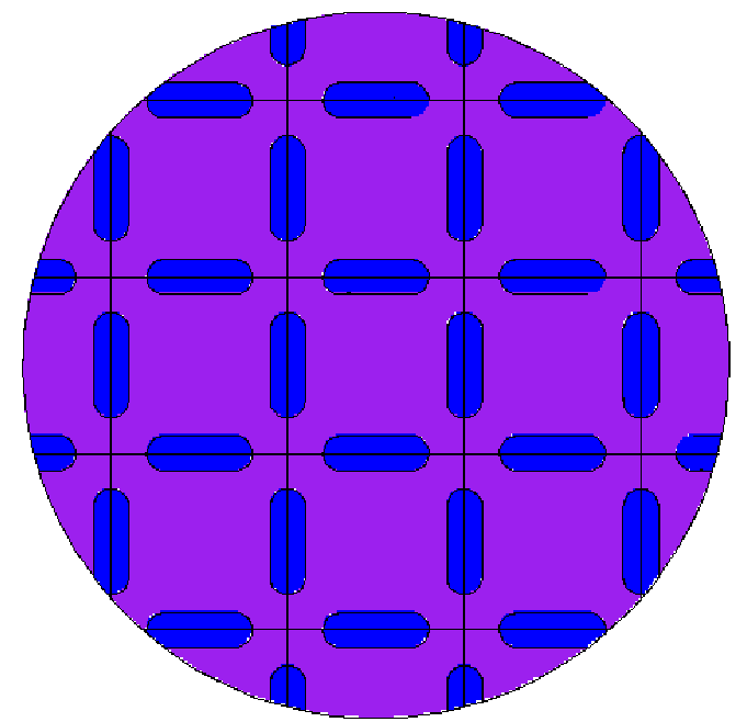
4.8.4 Lattice of a Lattice (LatticeOfLattice.cxx & LatticeOfLattice_serpent.cxx)
The purpose of this example is to illustrate a hexagonal Lattice of big structural hexagons, themselves filled with a hexagonal lattice of fuel rods (like in a SFR core)
-
//
// Material
//
Material *Iron=new Material();
Iron->SetDensity(7.87); //density in g/cm3
Iron->AddNucleus(26,56,1.);
Material *Na=new Material();
Na->SetTemperature(600);
Na->SetDensity(0.97);
Na->AddNucleus(11,23,1);
Material *Na_cold=Na->Clone(300); //just to see in Serpent all hexagons
Material *Fuel=new Material();
Fuel->SetTemperature(900);
Fuel->SetDensity(19.);
Fuel->AddNucleus(92,238,0.8);
Fuel->AddNucleus(94,239,0.2);
//
// data size
//
double VesselH=1.1; //the core size
double VesselR=1.1;
double FuelHexaSide=0.05; //(small) fuel hexagons side
double PinRadius=0.02; //fuel pin radius
double StructHexaSide=8./sqrt(3.)*FuelHexaSide; //(big) structure hexa
double StructThick=0.01; //the thickness of the structure (inner
// part of this structure is filled with
// FuelHexa.
//
// Shapes
//
//the Core
Shape_ptr Vessel(new Tube(VesselH,VesselR));
//the Exterior
Shape_ptr Exterior(!Vessel);
//the outside structure hexagon
Shape_ptr StructHexa(new Hexagon(VesselH,StructHexaSide+StructThick));
StructHexa->SetUniverse();
//the inside structure hexagon
Shape_ptr InnerStructHexa(new Hexagon(VesselH,StructHexaSide));
InnerStructHexa->SetUniverse();
// put the structure hexagons in the vessel
StructHexa>>Vessel;
//
//a "fuel hexagon"
//
Shape_ptr FuelHexa(new Hexagon(VesselH,FuelHexaSide));
FuelHexa->Rotate(-Pi/2);
FuelHexa->SetUniverse();
//put the fuel hexagons in the structure (inner part)
FuelHexa>>InnerStructHexa;
//
// Cells
//
PinCell *Reflector=new PinCell(); //Reflector=beetwen Core and big
Reflector->SetSurroundingMaterial(Na_cold); //hexagons. This is "cold Na" mat
PinCell *FuelHexaBorder=new PinCell(); //Fill the inner part of big
FuelHexaBorder->SetSurroundingMaterial(Na_cold); //hexagons with cold Na"
PinCell *Carandache=new PinCell(); //This is a fuel pin with
Carandache->AddLayer(Fuel,PinRadius); //a cylinder of fuel
Carandache->SetSurroundingMaterial(Na); //surrounded by Na
Cell *exterior=new Cell(Exterior,0,0); //out side of the core
exterior->SetComment("The exterior of the reactor");
Cell *vessel=new Cell(Vessel); //the core
vessel->SetComment("The reactor vessel");
Cell *innerstructhexa=new Cell(InnerStructHexa);
innerstructhexa->SetComment("The Inside struct Hexa");
Cell *exterior_innerstructhexa=new Cell(!InnerStructHexa,Iron); //space beetwen InnerStructHexa
exterior_innerstructhexa->SetComment("The Big Hexa claddings");//and StructHexa fill with Iron
LatticeCell *structhexa=new LatticeCell(StructHexa);
structhexa->SetComment("The Ouside struct of Big Hexa (lattice)");
int range1=int(VesselR/(1.5 * StructHexaSide)+1);
structhexa->SetLatticeRange(-range1,range1,-range1,range1);
double StructHexaWidth=sqrt(3.)*StructHexaSide;
for(int i=-range1; i<=range1; i++)
for(int j=-range1; j<=range1; j++)
{
int pos[3]={i,j,0};
double xt = StructHexaWidth * (i + j*0.5 ) ;
double yt = 1.5 * StructHexaSide * j;
double X[2]={xt,yt};
if(IsHexagonInTube(X,StructHexa,VesselR))
structhexa->FillLattice(InnerStructHexa,pos);
else
structhexa->FillLattice(Reflector,pos);
}
LatticeCell *fuel_hexa=new LatticeCell(FuelHexa);
fuel_hexa->SetComment("The fuel hexagonal lattice");
int range=int(StructHexaSide/(1.5 * FuelHexaSide)+1);
fuel_hexa->SetLatticeRange(-range,range,-range,range);
double FuelHexaWidth=sqrt(3.)*FuelHexaSide;
for(int i=-range; i<=range; i++)
for(int j=-range; j<=range; j++)
{
int pos[3]={i,j,0};
double xt = 1.5 * FuelHexaSide * i ;
double yt = FuelHexaWidth * ( j + i*0.5 );
double X[2]={xt,yt};
if(IsHexagonInHexagon(X,FuelHexa,InnerStructHexa))
fuel_hexa->FillLattice(Carandache,pos);
else
fuel_hexa->FillLattice(FuelHexaBorder,pos);
}
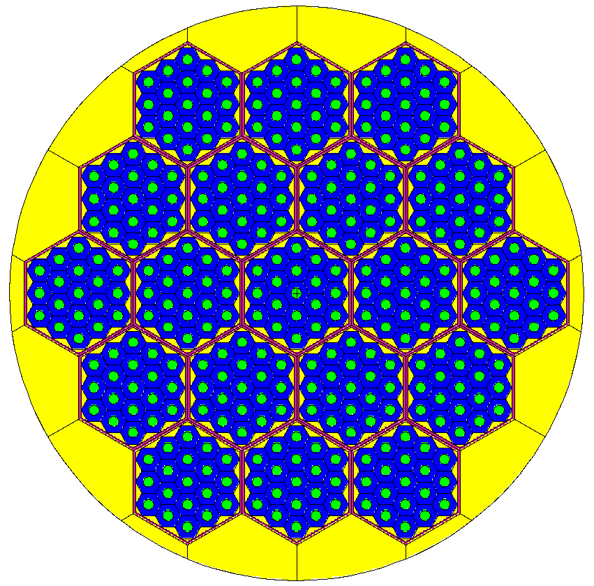
Chapter 5
Materials, Sources, Tallies, ...
5.1 Definition of material
A Material is a set of nuclei with their proportions (default units is %mol), it has a density and a temperature.
For example to define B4C of density 2.52 g∕cm3at 296 K:
-
Material *B4C=new Material();
B4C->SetDensity(2.52); //default units are g/cm3
B4C->AddNucleus(5,10,0.199); //Boron is composed 19.9% of 510B
B4C->AddNucleus(5,11,0.801); // and 80.1% of 511B
B4C->AddNucleus(6,0,0.25); // This is natural C (Z=6, A=0) ; for 1 mol of B one has 0.25 mol of C
Just before wrintting Material in MC file, proportions are normalized to 1. The Material::AddNucleus() method has the general form
-
Material::AddNucleus(Z,A,I,prop);
or
-
Material::AddNucleus(Z,A,prop);
where Z is an integer corresponding to the proton number of the nucleus, A, an integer for the number of nucleons, I, an integer for the isomeric state and prop, a double for the proportion of the nucleus in the Material. For natural isotopes A=0 ; for ground state I=0 (this is the default value when not specified). See § 5.1.3 for units.
-
A Material can contain one nucleus which is a “moderator”: this means that the special treatment S(α,β) is applied for low energy in MC run for this nucleus. In order to say that a nucleus is a moderator, one has to add a string for the last parameter of Material::AddNucleus (see 5.1.4.0.0 for a full description) ; defining thermal treatment for hydrogen in light water leads to:
H2O->AddNucleus(1,1,2.,kpMOL,"H2O"); //here the unit of proportion must be given explicitly
H2O->AddNucleus(8,16,1.);
5.1.1 Clone
A Material can be cloned via the Material::Clone(double Temperature) method. There are 2 types of clones depending on:
-
whether the material does not evolve and the Temperature argument of Material::Clone() is negative (the default) (see example of B4C_Light in § 5.1.7): the clone is only used because it makes possible to define a material with the same number in MCNP but also present at different densities in different cells. A call to Material::SetTemperature() will have no effect on such a clone!
-
or whether the material will evolve and/or the Temperature argument is positive or null (see example of Fuel2 and B4C_Hot in § 5.1.7): the clone is a “true” clone, i.e., all compositions and proportions are duplicated (2 different material numbers in MCNP). Of course the density, temperature,... of the clone could be changed after cloning, as well as new nuclei could be added. This kind of clone is the correct way to handle 2 evolving cells starting with the same composition but evolving independently. Note that by default the density of the clone is the one of the original material.
5.1.2 Mix (Mix.cxx)
Two Materials of different densities can be mixed together to create a third material. This is useful in many situations, e.g., the case of reactor fuels with a given enrichment of fissile isotopes. The principle is the following:
-
M12=M1->Mix(M2,part,kpMOL);
M12 is a new material and is created from the molar part mixture of materials M1 and M2 (for example Uranium and Plutonium Oxides). M1 and M2 can not be used in the problem, because the Material::Mix method forces them to be fictitious materials by using the Material::ForbidPrint() method: THIS IS DONE IN THE Material::Mix() METHOD. The density of the new material M12, is calculated as
where ωi and ρi are the mass fraction and density of material i. The temperature of the new material is the same as that of material M1.
5.1.3 Units
Density
Default units (k=constant, d=density) for density is kdGCM3 (g∕cm3); but, to avoid confusion, you must set the density unit in Material::GetDensity() (either kdGCM3 (g∕cm3), kdATCM3 (at/cm3) or kdATBCM (at/barn.cm)). User may give the density in atom/barn.cm by using Material::SetDensity(density, kdATBCM).
NOTE: If the density is not given (i.e. set to the default value 0), it could be automatically found if the proportions are given in atoms/barn.cm or in atoms/cm3 .
Proportions
Default units for proportions are in molar percentage. To give proportion in other units, use
-
Material::AddNucleus(Z,A,I,prop,UNITS)
where UNITS stands for (k=constant, p=proportion): kpMOL ("%mol" (default)) or kpMASS ("%mass" ) or kpATBCM ("at/barn.cm") or kpATCM3 ("at/cm3").
5.1.4 Material extension for MC
In MCNP or Serpent, material codes have extensions (like “.60c”). These extensions are very important because they distinguish isotopes at different temperatures, bases, versions,… In practice, if no extension is specified in MCNP file, the first isotope encountered in the xsdir is chosen regardless the temperature imposed in the cell where the material is (but this is not the case in Serpent). In MURE user has different ways to specify an extension.
-
This can be done manually for each nucleus of the material composition:
-
mat->GetNucleus(Z,A,I)->SetXSExtension(".49c")
-
-
This can be done manually for all nuclei of the material composition:
-
mat->SetDefaultXSExtension(".49c")
then each nucleus of the Material mat will have this ".49c" extension.
-
-
If the MCNP code for a particular Nucleus (Z,A,I) of a given Material mat is known, it can be specified by using:
-
mat->GetNucleus(Z,A,I)->SetXSExtension(".49c")
-
-
This can be done automatically (this is the recommended way): the specific file, the so-called “BaseSummary.dat” file, which contains xsdir/xsdata information written in a different way for search efficiency, is used. The extension is chosen according to the Material temperature. In fact the closest temperature to the one of the Material is chosen with the help of classes BasePriority and TemperatureMap. (see below)
-
If evolution is need, the automatic procedure is certainly required...but I am not sure (PTO).
-
If one specifies the extension value (either via Nucleus::SetXSExtension() or Material::SetDefaultXSExtension() or Nucleus::SetModeratorName()) then you must provide in the xsdir the corresponding data files.
S(α,β) Treatment and MT card
When the special treatment S(α,β) is desired for low energy, MCNP MT card arguments or Serpent moder and therm cards have to be specified. Consider the water example:
-
H2O->AddNucleus(1,1,2.,kpMOL,"H2O");
H2O->AddNucleus(8,16,1.);
-
this can be done manually: the string “H2O” must not be empty ; then
-
H2O->GetNucleus(1,1)->SetModeratorName("lwtr.01t");
-
-
this can be done automatically: the BaseSummary.dat file is read to find the code of S(α,β) treatment file ; this time, because S(α,β) treatment is material dependent, the string has to refer to a given ”Category” to specify which kind of effects are taken into account ; in the above example, hydrogen has different S(α,β) treatment for light water, polyethylene, benzene, ... The complete list of available Categories is given in Nucleus in the Nucleus::SetModeratorCategory():
H2O for H in light water H/Zr for H in ZrH poly for H in polyethylene D2O for D in heavy water BeO for Be in Be oxide Be for Be in Be metal Gr for graphite Zr/H for Zr in ZrH The moderator category can also be any real MT file name such as “lwtr” or “u/o2”, ...
5.1.5 Pseudo Materials
PseudoMaterials are particularly useful for thermal-hydraulics problems. Normally, the material temperature dictates which extension (e.g. “.60c”) for cross-sections will be used from the evaluated data libraries. The default behavior in MURE is that the nearest available temperature is used, the maximum tolerable difference between this temperature and the desired material temperature being defined in the TemperatureMap class. However, there are occasions where it is useful to perform a stochastic interpolation at the desired temperature by adding two identical nuclei at different temperatures in the material in varying proportions. These types of materials are called PseudoMaterials, because, in principle, they behave as a material at a precise temperature, T, even though the cross-sections in the evaluated data libraries at this precise temperature do not exist. To declare a Material (Mat) to be a PseudoMaterial requires the following simple line:
-
Mat->SetPseudoMaterial();
From this point onward, MURE will automatically create two identical nuclei with different extensions/temperatures and in the correct proportions for, every nucleus which is added to this material. No other commands are necessary. However, in the case of an evolving material (a reactor fuel rod for example), this can cause the addition of many, many extra nuclei to the material, thus slowing down MCNP calculations by perhaps as much as 20%. In the case that the user only wants to declare certain nuclei to be PseudoNuclei (for example, the most important ones, such as the fissile and fertile nuclei) the following kind of lines can be added after the creation of a Material:
-
UO2Fuel->AddNucleus(92,235,0.04);
UO2Fuel->AddNucleus(92,238,0.96);
UO2Fuel->AddNucleus(8,16,2.0);
UO2Fuel->GetNucleus(92,235)->SetPseudoNucleus();
UO2Fuel->GetNucleus(92,238)->SetPseudoNucleus();
Now, only the selected nuclei will be treated as pseudo nuclei and automatically inserted twice into the MCNP file at the two nearest data base temperatures in the correct proportions. The proportions, ω1 and ω2 , for the interpolation are calculated in the following way:
where T1 and T2 are the nearest two temperatures in the evaluated data base files straddling the desired temperature T.
5.1.6 MC material Printing
This section concerns only evolving Materials. When evolution is required, at the beginning, many nuclei are present in the material but in a very small proportion. Each time a neutron enters in a cell, MC code tries to find the nucleus on which the potential reaction could happen. Thus, the more complex is a material, the longer is the MC run. The idea is to suppress only for the MC print, the nuclei which do not contribute “significantly” to neutron transport to save CPU time. The criterion is based on the evaluation of total cross-section σT and nucleus proportion p. If a nucleus of a material has a p × σT < 𝜀, it is not printed. The value of 𝜀 is by default set to 0.1% × 1mb = 10−6. This can be changed via MURE::SetMCNPNucleusThreshold(). To be noticed that perturbative tallies of all evolving nuclei are written (in order to evaluate the cross-section...). The effect of this procedure is thus to accelerate MC runs at the beginning of the evolution where time steps between MC are generally smaller, and add more and more nuclei as far as the evolution is going on (with larger time steps between MC runs).
5.1.7 Examples
Please take a look at Material_test.cxx and Material_test2.cxx and the corresponding Serpent version for the second one. The use of Nucleus::SetXSExtension or Material::SetDefaultXSExtension supposed that the user provide a correct xsdir file with all necessary information.
5.1.8 Automatic extension finding
Here is a short description of the automatic nucleus extension finding.
Making the BaseSummary.dat file
In order to work, a specific file, BaseSummary.dat, must be present in the data directory. The aim of this file is to facilitate the search for a given Z,A,I and related xsdir/xsdata information (see also § 1.4.2 and 1.4.3).
Extracting the MC nucleus code from the BaseSummary.dat file
Suppose the desired ZAI exists in the BaseSummary.dat file. Then the choice of the desired nucleus is based on 2 criteria: the first one is related to the preference in a nuclear base (ENDB, JEFF, JENDL) and the version of this base, and the second criterion is related to the nucleus temperature. A score is calculated for each criterion, and the best score is chosen. Two classes are in charge of these criteria: BasePriority and TemperatureMap.
-
BasePriority class: a priority base is organized in 3 levels (base names) and maximum 3 sub-levels (base versions). Level 1 has a greater priority than level 2 and so on. By default, the 3 levels are: (1) ENDFB (USA), (2) JEFF (European) and (3) JENDL (Japan). Only 1 sub-level is defined for each base (6.1 for ENDFB, 3.0 for JEFF and 3.3 for JENDL). If a user defines for each level the same base (e.g., (1) ENDFB, (2) ENDB, (3) ENDB), then this imposes the base choice (i.e., no other choice is possible).
For example
-
BasePriority *BP=new BasePriority();
BP->SetBasePriority(0,"JEFF"); //1st prefered base
BP->SetVersionPriority(0,"3.1",0); //1st prefered version for 1st prefered base
BP->SetVersionPriority(1,"2.2",0); //2nd prefered version for 1st prefered base
BP->SetBasePriority(1,"ENDFB"); //2nd prefered base
BP->SetBasePriority(2,"JENDL"); //2nd prefered base
gMURE->SetBasePriority (BP);
will choose nuclei first in JEFF 3.1, the if not found, in JEFF 2.2, then in JEFF (what ever is the version), then in ENDFB (default first preferred version VI.8) and then in JENDL (default first preferred version 3.3).
If one want to impose nuclei in ENDFB VII.0, then user should do
-
BasePriority *BP=new BasePriority();
for(int i=0; i<3; i++)
{-
BP->SetBasePriority(i,"ENDFB");
for(int j=0; j<3;j++)-
BP->SetVersionPriority(j,"7.0",i);
-
}
gMURE->SetBasePriority (BP);
-
In that case, only nuclei given in the wanted nuclear base are used.
-
-
TemperatureMap class: this class defines a temperature “binning” T[i] and a precision ΔT ; an input temperature Tin can be searched in this binning with respect to the precision. For example, if T[0] = 300K, T[1] = 500K and ΔT = 50K, then all Tin in [250K,350K] will have a score of
![|Tin−T[0]| ΔT](UserGuide3x.png) , all Tin in [350K,450K] will have a 0 score. The precision ΔT can be set via gMURE->GetTemperatureMap()->SetDeltaTPrecision(). A zero score in temperature stops the MURE execution: you may either increase the ΔT precision or build the nucleus data file (ACE format) at the desired temperature.
, all Tin in [350K,450K] will have a 0 score. The precision ΔT can be set via gMURE->GetTemperatureMap()->SetDeltaTPrecision(). A zero score in temperature stops the MURE execution: you may either increase the ΔT precision or build the nucleus data file (ACE format) at the desired temperature.
5.1.9 Automatic XSDIR construction
Using the extension finding, MURE can build the XSDIR/XSDATA file that is used by MC code to get the cross-sections used in the problem. To use this option, you just have to set :
-
gMURE->SetAutoXSDIR();
When getting the code for MC file, MURE will then save the best line it finds in BaseSummary.dat. Therefore, right before building the MC file (the XSDIR is built at the first step of an evolution), MURE will build the XSDIR/XSDATA file by using all these best lines it saved.
IMPORTANT : If an existing XSDIR/XSDATA is already present in the MC run directory, then MURE will NOT build a new one ; the existing one will be used by MC code. Thus either the xsdir/xsdata is correct, either you have to remove it.
5.2 Particle Source
Because the difference between particle source definition in MCNP and Serpent is great, MURE source definition uses 2 different classes, MCNPSource and SerpentSource to avoid confusion for the user ; they are sibling of the MCSource class.
The MCNPSource SerpentSource classes enable the definition of particle sources (up to now only neutron sources may be defined for Serpent). Nevertheless, some source definition methods are common to both classes. Two type of source can be defined, source for criticallity calculation (called kcode mode) and fix sources for non fissile or subcritical system only. For Serpent, source possibilities are much more simpler than for MCNP ; in MURE, the source implementation for Serpent is also much less developed. Mainly position and energy of punctual monoenergetic isotrope source can be defined. Criticallity is defined also by the “SerpentSource::SetKcode” method. In the following section, the MCNPSource is used because of its greater complexity, but looking to SerpentSource methods and their analog counterpart in MCNPSource is self understandable.
The source may be defined with MCNP card or as an external source. In the latter case (MCNPSource::SetExtern()), external source will be read in a special file. This is valid in subcritical mode as well as in critical (KCODE) mode (not true for Serpent). One chooses to run in subcritical mode (default) or in KCODE mode via the MCNPSource::SetKcode() method.
5.2.1 Setting Source for MURE
Once an MCSource has been defined, one has to give this source to MURE class:
-
MCNPSource *mysource=new MCNPSource(1000); //1000 source particles
gMURE->SetSource(mysource);
5.2.2 Criticallity calculation: Kcode mode
To be noticed that, for Kcode, the number of source particles defined in the constructor of MCSource is in fact the number of neutrons per cycle.
To initiate a KCODE, a SDEF (or KSCR) card is needed (if no external source is given!). By default in MCNP, the position of this initial source is (0,0,0). If you want to change the source position, use the MCNPSource::SetPosition(). In Serpent the default positions are chosen in cells containing fissile materials.
-
MCNPSource *mysource=new MCNPSource(1000); //1000 source particles/cycle
//Kcode with first expected keff=1, 10 inactive cycles and 80 active ones
mysource->SetKcode(80,10,1);
gMURE->SetSource(mysource);
If one want to use a source from a previous KCODE:
-
mysource->UsePreviousRunSource(“olds”);
where the source file olds is the result of a previous run. In case of evolution, if you do not specify any argument, the source will be calculated as specified by inactive cycles, and then for next MCNP runs, the source is taken from the previous cycle.
5.2.3 More elaborated sources (MCNP only)
The MCNPSource gives more details on MCNPSource class possibilities. Two simple examples are presented:
First
-
MCNPSource *source=new MCNPSource(1000); //1000 particles per cycle
source->SetKcode(500,20,1); //critical mode (500 active cycles, 2O inactive, supposed keff=1)
source->SetKSRC(); //use fission spectrum for neutron energy
source->AddPosition(0,0,0); //add one position for the source at (0,0,0)
source->AddPosition(0.1,0.1,0.1); //add an other one at (10cm,10cm,10cm)
source->AddPosition(0,0,0.2); //add an other one at (0,0,20cm)
source->AddPosition(0,0,-0.2); //add an other one at (0,0,-20cm)
and the second
-
MCNPSource *source=new MCNPSource(); //SDEF source with 10000 particles
source->SetEnergie("D1"); //energy is define by the source probability 1
source->SetDistribution("RAD=D2 EXT=D3"); // radial and axial extension are
// defined by source information 1 and 2
source->AddBias("SP1 -5 2.0"); //p(E)=E*exp(E/2.MeV)
source->AddBias("SI2 1. 2."); // radial extension from r=1cm to r=2cm
source->AddBias("SI3 -10. 10.");// axial extension from z=-10cm to z=10cm
5.2.3.1 Source define via Spectrum class (MCNP only)
One can define energy distribution source using the Spectrum class and the MCNPSource::UseThisEnergyDistribution() method. Any call to that method will dump in MCNPSource_YourEnergyDistribution.dat, the ASCII spectrum of this source (for user own use) as well as the total number of particles emitted (for normalization purpose).
To be noticed: this method will change the source particle type according to the Spectrum type (neutrons for NeutronSpectrum, γ for GammaSpectrum, …).
This method only change energy distribution of the source (using MCNP distribution source cards (D, SI, …) numbered by default from 800).
5.2.3.2 Tube Source (MCNP only)
It is possible to define volumic cylindrical sources with the help of the Tube class. Two methods are available : MCNPSource::AddTubeSource(Tube *tube, string energy) and MCNPSource::AddTubeSource(Tube *tube, Spectrum *spectrum). In both cases, the tube is used to define the shape of the source. The first one allows to use either mono-energetic sources or using source distributions “D” card. In the latter case, the user need to provide himself the distribution description via the MCNPSource::AddBias() method (see TubeSource.cxx example). The method using Spectrum class argument use Spectrum to define both particle type of the source (neutrons for NeutronSpectrum, γ for GammaSpectrum, …) and energy spectrum (see TubeSource2.cxx example).
Theses 2 methods use internally source distribution cards (D, SP, SI, …). The starting number of these distribution is 900. Thus don’t use number above 900 to define your own source distribution and biasing.
Of course you can add more than one Tube source ; but it is only possible to add more Tube sources with same calling method (either MCNPSource::AddTubeSource(Tube *tube, string energy) or MCNPSource::AddTubeSource(Tube *tube, Spectrum *spectrum). One cannot mix them.
5.2.3.3 Define MCNP Source from the result of an evolution (MCNP only)
If one want to use the energy distribution of a spent fuel which has cooled for a time t, use MureGui and dump the source in a MURE format (“Save Data” button, then select the “MURE INPUT Spectrum” radio widget). The generated file can be inserted in a MURE “cxx” code (c.f. MureGui section 8.3.6).
5.3 Tally class
The Tally class enables tallies for MCNP/Serpent to be defined.
WARNING : NEVER USE : “Tally *f=new Tally[N]” BUT USE INSTEAD “vector<Tally*> f(N) ; for (int i=0 ; i<N;i++) f[i]=new Tally;”. The reason is that when tallies are deleted, one need
to use either “delete []” or “delete” ; in MURE, the second case is chosen which is incompatible with the former declaration.
MCNP tallies or equivalent Serpent detectors are used to store quantities from a run ; Serpent detectors and MCNP tallies have lots of common points but the MCNP version has more possibilities (Group tallies, tally normalization, ...). The implementation of tallies in MURE is (at least for historical reasons) much more developed for MCNP. Nevertheless, surface tallies (type 1 and 2 in MCNP) are not fully implemented (Surface calculation, ...) even if one can use them with special precaution/verification.
There are 2 main tally types: Surface tallies (type 1 and 2 in MCNP, same convention is kept for Serpent) and Cell tallies (4,...). At present, only Cell tally of type 1 (current through a surface), 2 (flux through a surface), 4 (flux in cell), 6 (energy deposition in a cell) and 7 (fission energy deposition in a cell) are implemented in MURE. Surface tallies have not been tested at all and stochastic surface calculation is not implemented in MURE.
A Tally consists of
-
a tally type (what is the desired quantity, e.g. flux in a cell),
-
a list of TallyBin: this may be SimpleBin (a cell or surface number), GroupBin (a group of cells or surfaces) or a LatticeBin which allows to obtain tallies in cells with universes. The GroupBin does not exist in Serpent ; the LatticeBin is not implemented in MURE for Serpent.
-
a Time and/or Energy binning (linear, log or arbitrary binning)
-
a list of TallyMultiplicator (Tally Multiplicator) that allows to obtain cross-sections, .... A TallyMultiplicator is composed of a multiplicative constant, a material number and a Reaction. The multiplicative constant is not used in Serpent.
Of course Cell tally bin types could not be mixed with surface tally bin type. Tally bins are added with the Tally::Add() method (for cell/surface bins) whereas energy and/or time bins are added with Tally::AddEnergy() or Tally::AddTime().
Tally multiplicator may be added with Tally::AddMultiplicator() to obtain cross sections, reaction rates and so on.
Example of Tallies:
-
Tally *t1=new Tally(); //default tally type is 4: flux in cell
t1->Add(cell_1);
t1->Add(cell_2);
LatticeBin *lpb=new LatticeBin(rod); //rod is a cell associated to an element of a Lattice
lpb1->AddContainer(core); //core is a cell fills by "rods"
t1->Add(lpb);
t1->AddEnergy(1e-2,1.e7); //log energy binning from 0.01 eV to 10 MeV with 10 bin/decade (default)
t1->AddMultiplicator(mat_1,new Reaction(102)); //capture reaction rate
t1->AddMultiplicator(mat_1,-6);//fission reaction rate
When in LatticeBins, you can precise the positions of the cell in the lattice, use a string which gives the position in the MCNP way, that is :
-
string pos="[0 0 0]";
LatticeBin *lpb=new LatticeBin(rod); //rod is a cell associated to an element of a Lattice
lpb->AddContainer(core,pos); //core is a cell fills by "rod" (e.g. a lattice)
This means that you are interested by the flux in the cell rod which is in the cell core at the lattice position [0,0,0]. The result in MCNP file will be (given that the number of cell rod is 1 and cell core is 2):
-
F4:N (1<2 [0 0 0])
Finally, you can use the universe shorthand (u=1 for instance), simply by giving the universe number, either directly if you know it or by using Shape::GetUniverse() :
-
Tally *t1=new Tally();
t1->Add(MainShape->GetUniverse());
Please note that, in MCNP, the universe shorthand doesn’t work for lattice elements filled with the universe number, that is to say, when a lattice is filled by position, for instance when in MURE we use Cell::FillLattice(Universe_Number, Position), the universe is not detected by MCNP. (see example Tally_Test.cxx)
As this shorthand is replaced by all the cells filled with the universe, we strongly recommend that you use it only if you are perfectly sure of the number of cells involved in the tally defined in that way.
Each tally must have a definite volume (or surface). The volume is set via the Tally::SetBinVolume() or for a given bin, via the TallyBin::SetBinVolume() or TallyBin::SetVolume(). This may be done manually or automatically: if no bin volume has been provided, the volume is automatically calculated by a stochastic method (see also the note C.1 concerning the volume calculation). For lattices and universe shorthand, as multiple volumes are needed for each bin, the SetBinVolume() method precises a partial number.
-
Tally *t1=new Tally(4);
t1->Add(Cell1);
t1->SetBinVolume(0,1.e-6,0); // Set the volume of Cell 1 to 1 cm3
LatticeBin *lpb2=new LatticeBin(rod1);
lpb2->AddContainer(rod2);
lpb2->AddContainer(core);
Tally *t2=new Tally(4);
t2->Add(lpb2); // A Lattice Bin giving somthing like (1 2 < 3)
t2->SetBinVolume(0,1.e-6,0); // Set the volume of Cell 1 in cell 3
t2->SetBinVolume(0,1.e-6,1); // Set the volume of Cell 2 in cell 3
The partial number follows the order of the output. (to know exactly the order for lattice bin volumes, see MCNP doc or example Tally_test.cxx).
5.3.1 Fluence to dose conversion (MCNP Only)
The Tally::AddFluenceToDoseConversion() method converts fluence (only for F4 type tally) to dose rate (rem/h) using fluence to dose conversion factors. It can be use only for photons or neutrons. The conversion factor are store in /path_to_mure/MURE/data/GammaFluenceToDose.dat and NeutronFluenceToDose.dat (they are taken from [23]). Interpolation is done for energies and for factors. This interpolation is done by default in log way. The 2 boolean parameters of Tally::AddFluenceToDoseConversion() allows to specify linear interpolation for energy (the 1st one) and conversion factors (the 2nd one).
-
Tally *MyTally=new Tally(4,ParticleType);//fluence to dose works only for ParticleType=”P” or “N”
MyTally->Add(....);
MyTally->AddEnergy(.....);
MyTally->AddFluenceToDoseConversion();
Chapter 6
Nuclei Tree
6.1 Nuclei Trees: general considerations
To evolve a given material, it is essential to know in advance the ensemble of nuclei which it can produce via successive nuclear reactions and decays. This information comes from the Nuclei Tree object, which is defined by the NucleiTree class, and contains the linking information between all the nuclei that exist in the chart of nuclides. Nuclei can be transformed into other nuclei by nuclear decays (β, α, electron capture, etc.) and nuclear reactions ((n,γ), (n,2n), fission, etc.). In general a particular nucleus has daughters (those nuclei it can transform into) and parents (those nuclei that can produce it). To calculate how much of a particular nucleus is produced during the evolution it is essential to know the ways in which it can be produced and the ways it can be destroyed.
We cannot only define the total global nuclear tree (the connections between all 3834 nuclei), but also the local or particular tree for a given nucleus. The particular tree for a certain nucleus is, in general, a subset of nuclei and their linking from the global tree. To extract an individual tree from the global tree, the NucleiTree::ExtractZAI method is used. The local tree is explored recursively by starting at the given nucleus (see figure 6.1) and then finding each successive reaction and decay daughters.
6.1.1 How the tree information is stored
-
The global nuclear tree has a vector of all the physically possible ZAI objects, representing the different isotopes, including long-lived isomers of the same isotope, as an attribute. Each ZAI object contains vectors of pointers to other ZAI which are either its reaction daughters or its decay daughters. When a particular tree is extracted, the parental relations are also determined (see figure 6.2). It is then possible to follow the tree by jumping from ZAI to ZAI, and to understand for each ZAI object all the ways it can be created and destroyed.
6.1.2 Cutting or simplifying the tree
Isotopes in the chart of nuclides have half-lives ranging over ~40 orders of magnitude. In a reactor core neutron fluxes are much lower (∼ 1015 neutron/cm2/s) than in supernova explosions (up to ∼ 1024 neutrons/cm2/s) and thus decay rates are usually much higher than reactions rates for most short-lived nuclei. Furthermore, the reactor fuel composition only changes significantly after some years, so short-lived isotopes play no important role in the evolution. We can therefore assume that nuclei with short half-lives decay instantaneously which allows us to simplify the tree and reduce the number of nuclei in the calculation and hence the calculation time. To simplify a nuclear tree requires these short-lived nuclei to be cut out of the tree and their reaction/decay parents and daughters re-linked into the tree correctly. There are two types of simplification for a particular tree branch, depending on whether the nucleus X in question is produced via decay (see figure 6.3) or nuclear reaction (see figure 6.4) .
Note that this means that in some cases a single type of reaction can produce multiple daughters with different probabilities (branching ratios), since the reaction daughter had more than one decay daughter itself, and was cut out of the tree because its half-life was too short (see figure 6.4). After the simplification process, these reaction daughters will have weights which are proportional to the decay branching ratios of the nucleus that was removed from the tree.
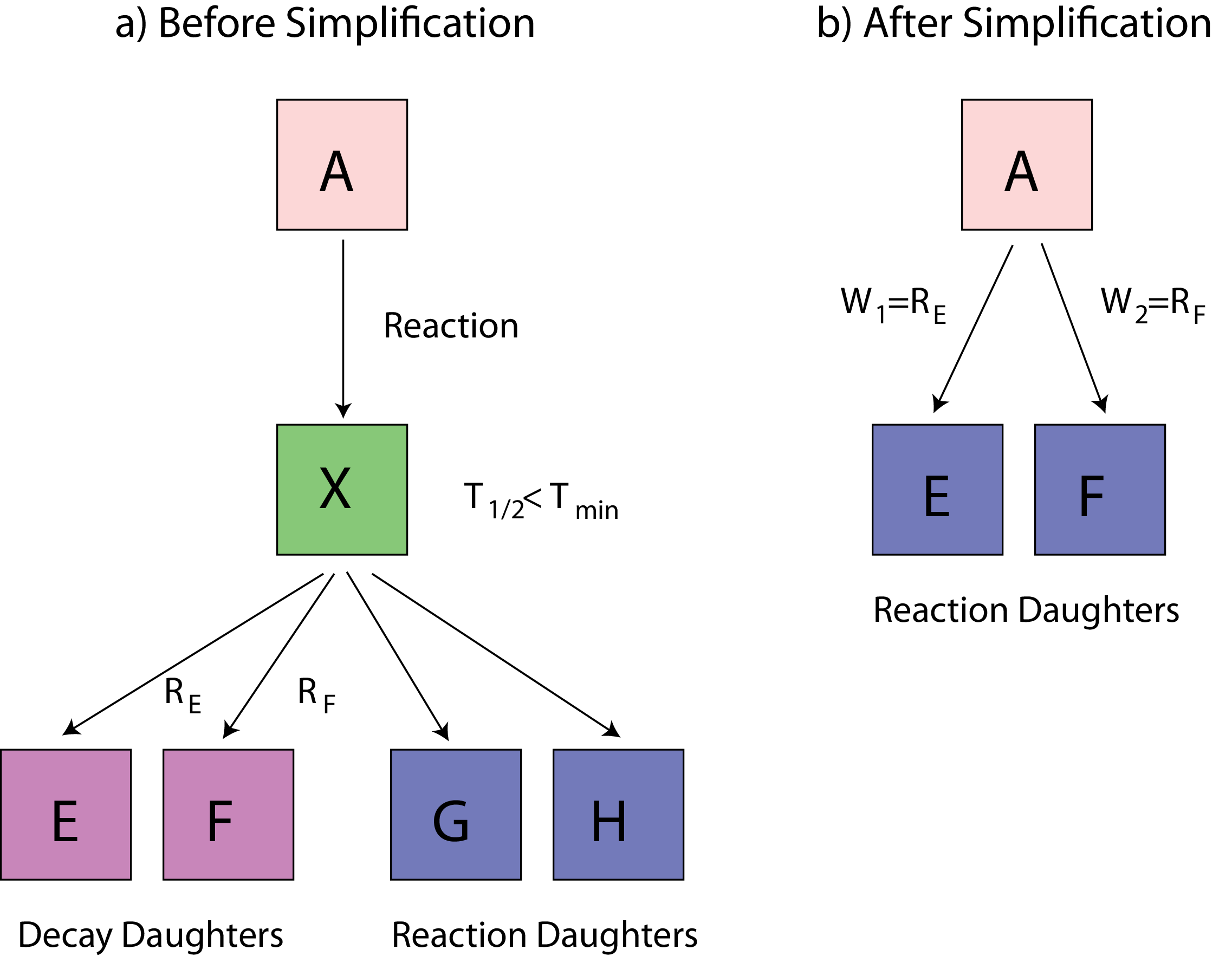
For a particular tree many nuclei towards the neutron drip-line end up getting cut out due to their progressively shorter half-lives. In figure 6.5 we can see the nuclei explored and then removed from the tree right up to the edge of the nuclear chart.

6.1.3 The difference/similarity of material trees
Two nuclei X, and Y will have identical trees if there is a pathway of decays and reactions that produces Y from X and also a pathway of decays and/or reactions that produces X from Y. Reactions (n,γ) and (n,2n) move up/down in mass, and decays only move down in mass. Once the mass is sufficiently low that (n,2n) reactions are not permitted, then decays will only take nuclei as far as the valley of stability and a stable nucleus are reached. At this point the tree branch ends. However, successive neutron captures are always possible, therefore fuels containing lighter elements, such as the Oxygen in Uranium Oxide (UOX) fuel, will have a different tree from a pure fuel’s one such as the 232Th (see figure 6.6).
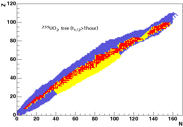
6.1.4 How many nuclei need to be considered in the evolution?
In all the previous chart figures, the reactions taken into account are: if Z < 50, (n,γ), if Z < 90, (n,γ) and (n,2n), and if Z ≥ 90, (n,γ) and (n,2n) and fission reactions. In reality, of course, nuclear cross sections are only available for a subset of all nuclei. Figures 6.7 and 6.8 show the nuclei with available reaction data found in the default MCNP4 cross-section (from ENDFB base). All the available reactions are plotted in figure 6.9.
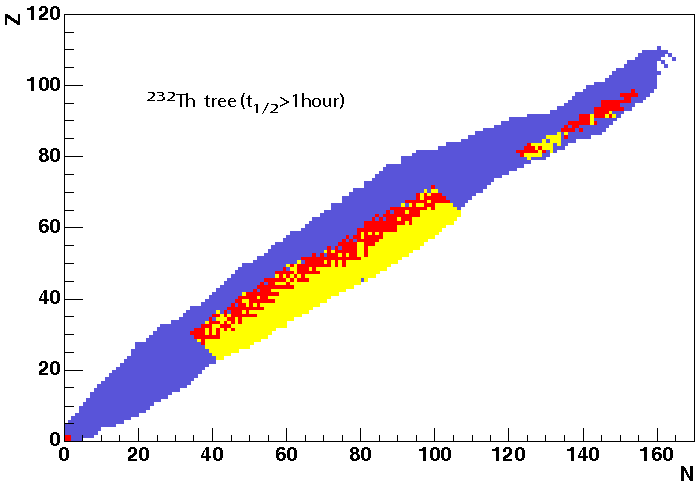
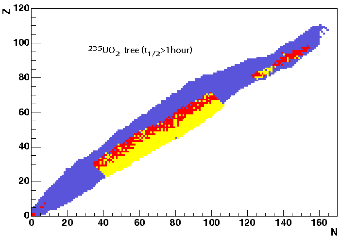
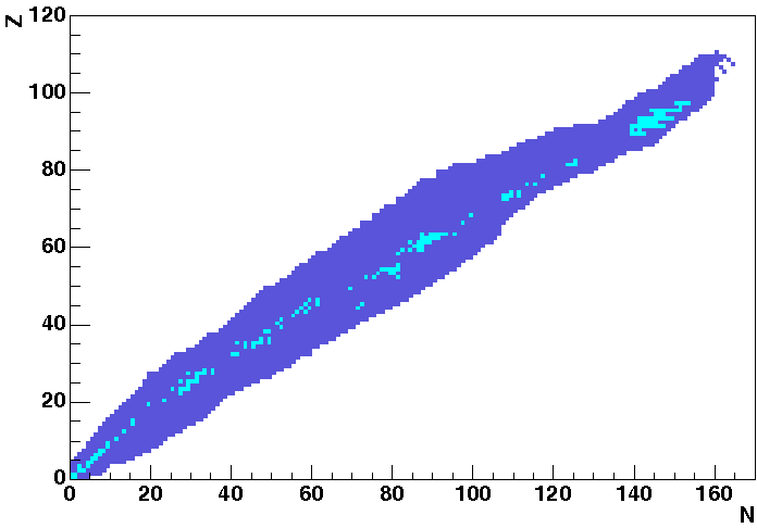
For a realistic half-life cut, the actinide nuclear tree still contains several hundred nuclei. However, simplification has reduced considerably the complexity of the problem(see figure 6.10)1.
6.1.5 Fission Products
Fission products are built according to the fission yields available in nuclear data libraries (default library is ENDF B 6.8). Fission yields are read in the FPyield.bin with the help of FPavailable.dat files (in the data directory). These files have been generated using SMURE/source/utils/fp/GenerateFPYield2 and can be regenerated using any ENDF fission product yields of ENDFB.X, JEFF.X, JENDL.X, etc libraries.
To be noticed, that for a given heavy nuclei, if the FP yields are not available, the “closest” Z,A,I heavy nuclei FP yields are used (which is of course wrong but probably better than nothing). For example, spontaneous fission of 244Pu uses the fission product distribution of the induced fission of 243Am. If some FP of the libraries are not included in the decay data file (chart.jeff3.1.1), then this fission product is ignored or, for isomeric states, the yield is given to first state below. Up to January 2024, the only case found is the production of the second isomeric state of 116Ag found in JEND4 and JENDL5 which the yield is added to the one of the first isomeric state of this nucleus.
They are the major contributor to nuclei increased in the reaction tree. The more FP in nuclear libraries, the longer the MCNP/Serpent execution time will be due to the increase in tally number. Thus, in order to obtain a first approximation, it may be convenient to run only a selection of fission products that may be considered as “fundamental”. We provide a method, NucleiTree::FissionProductSelection() to choose the most important FP. All other FP will not evolve (no resolution of Bateman equations) but instead are added in the real materials of the MC input file in order to have a good flux description. A default selection has been entered with the nuclei of Table 6.1 ; nevertheless the user can provide a file with its own selection. To use this selection you must use gMURE->KeepOnlyFissionProductSelection() ; to give your own selection, use gMURE->KeepOnlyFissionProductSelection(“MyFPSelection.dat”) where the file MyFPSelection.dat is an ASCII file with each FP you prefer to keep for evolution : for example
-
Z1 A1
Z2 A2
...
|
|
|
|
|
|
|
| 36-Kr- 83 | 46-Pd-107 | 54-Xe-134 | 60-Nd-145 | 62-Sm-152 | 66-Dy-160 |
|
|
|
|
|
|
|
| 40-Zr- 93 | 46-Pd-108 | 54-Xe-135 | 61-Pm-147 | 63-Eu-151 | 66-Dy-161 |
|
|
|
|
|
|
|
| 42-Mo- 95 | 47-Ag-109 | 54-Xe-136 | 61-Pm-148 | 63-Eu-152 | 66-Dy-162 |
|
|
|
|
|
|
|
| 43-Tc- 99 | 48-Cd-113 | 55-Cs-133 | 61-Pm-149 | 63-Eu-153 | 66-Dy-163 |
|
|
|
|
|
|
|
| 44-Ru-101 | 49-In-115 | 55-Cs-134 | 62-Sm-147 | 63-Eu-154 | 66-Dy-164 |
|
|
|
|
|
|
|
| 44-Ru-103 | 51-Sb-125 | 55-Cs-137 | 62-Sm-148 | 63-Eu-155 | 67-Ho-165 |
|
|
|
|
|
|
|
| 44-Ru-106 | 52-Te-127 | 55-Cs-135 | 62-Sm-149 | 64-Gd-155 | 68-Er-166 |
|
|
|
|
|
|
|
| 45-Rh-103 | 53-I -127 | 56-Ba-138 | 62-Sm-150 | 64-Gd-156 | 68-Er-167 |
|
|
|
|
|
|
|
| 45-Rh-105 | 53-I -135 | 59-Pr-141 | 62-Sm-151 | 64-Gd-157 | |
|
|
|
|
|
|
|
| 46-Pd-105 | 54-Xe-131 | 60-Nd-143 | 64-Gd-154 | 64-Gd-158 | |
|
|
|
|
|
|
|
6.1.6 Isomer Production from neutron reactions
TO BE NOTICED: Before July 2012, MURE only takes into account the case of 241Am. In the previous treatment, all ground state production was replaced by 242Cm ; this was of course wrong and lead to an over estimation of 242Cm production and an under estimation of 242Pu. This has been corrected since July 2012.
In some cases, neutron reactions like (n,γ), (n,2n) or other reactions can lead to either ground state or isomeric states of a nucleus. From all the many isomeric levels only the long-living are of interest, because for neutron physics application the isomeric state behaves like a new isotope with different half-live, reaction and decay channels. For example, let’s take the case of 241Am. Neutron capture on this nucleus leads to 242Am(T1∕2 ∼ 16h) and 242mAm(141y). Ground state decays in 242Pu(17.3%) by electronic capture and in 242Cm(82.7%) by β− decay. A file (IsomerProduction.dat) is provided to give the branching ratio (for thermal and fast spectrum) to produce its ground and isomeric states of a large set of nuclei. The format of this file is
-
ZtAtIt ZpApIp ReactionCode BRthBRf halflife Cutflag
for any isomeric state branching of a nucleus, where Z, A, I are proton number, mass number and isomeric state number, respectively. Subscripts t and p indicate target and product nuclei. The ReactionCode denotes the ENDF MT reaction number and BRth and BRf are the branching ratios averaged over a thermal (th) and fast (f ) neutron spectrum. 6.2 shows as an example the production (index p) of Am-242m from target (index t) isotopes 241Am, 242Am, 243Am, 244Am via the capture (102), inelastic scattering (4), n2n (16), n3n (17) neutron reactions, respectively. The branching ratio is given for a thermal LWR neutron spectrum (index th) and a fast spectrum (index f ).
|
|
|
|
|
|
|
|
|
|
| Zt | At | It | Zp | Ap | Ip | ReactionCode | BRth | BRf |
|
|
|
|
|
|
|
|
|
|
|
|
|
|
|
|
|
|
|
|
| 95 | 241 | 0 | 95 | 242 | 1 | 102 | 0.13 | 0.15 |
|
|
|
|
|
|
|
|
|
|
| 95 | 242 | 0 | 95 | 242 | 1 | 4 | 0.09 | 0.06 |
|
|
|
|
|
|
|
|
|
|
| 95 | 243 | 0 | 95 | 242 | 1 | 16 | 0.26 | 0.26 |
|
|
|
|
|
|
|
|
|
|
| 95 | 244 | 0 | 95 | 242 | 1 | 17 | 0.24 | 0.25 |
|
|
|
|
|
|
|
|
|
|
The “halflife” parameter is the half life of the produced ground state (T1∕2 ∼ 16h for 242Am) followed by its unit (here “h”) ; this parameter in not used, it is just an indication that can help the user to decide if the last parameter (CutFlag) is a “X” or a “M”. “M” means that MURE decide what to do according to MURE::GetShortestHalfLife() method. “X” forced the replacement of the ground state (e.g. 242Am) by its decay daughters. To be noticed, if “M” is chosen, wrong results can be obtained in 242Pu and 242Cm for example, if no cross section is available for the ground state (242Am). Currently, the mechanism of “X” and “M” is disabled and MURE handles everything according to MURE::GetShortestHalfLife().
Branching Ratio To use the branching data the corresponding reaction type must be available in the Ace Monte-Carlo library. This might be not the case for some total reactions like inelastic scattering which is the sum of all inelastic levels and continuum stored as MT 51–91. To generate this table, the nuclear data processing code PREPRO [24] is used to generate one group activation cross sections for any isotope of the TENDL 2014 [25] nuclear data evaluation. In PREPRO, the weighting spectrum options of the NJOY [26] code for spectrum type 5 (EPRI CELL) LWR and type 8 fast neutron spectrum were applied. In total, 30562 reactions of almost 3000 isotopes leading to isomeric states are generated. In the course of the depletion calculation MURE requests reaction rates from the MCNP run and applies the branching ratios depending on the target and production isotope to fill the transmutation matrix.
As another source for branching ratios for isomer production the nuclear data service at NNDC-ENDF maybe used, in the “advanced” or “extended” retrieval tab, by choosing “n,g” in the Reaction line and “MRNP” (Multiplicities for production of radioactive elements, MF=9) in the Quantity line. The branching ratio given in MURE/data/IsomerProduction.dat are effective branching ratio computed on a typical thermal and fast spectrum as explained in [27]:
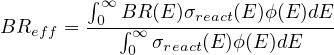
The NNDC-ENDF site gives either the branching ratio to the ground state or to the isomeric state(s) ; in MURE only one branching ratio maybe given (e.g. to the first state), the ground state ratio is then added. However, sometimes more than one branching ratio is needed. In that case, all ratios and reactions have to be added to the file. 2.
6.2 Nuclei Tree: the implementation
6.2.1 Important files
All provided data files are located in MURE/data. One can use either, gMURE->SetDATADIR(path) or the environment variable DATADIR (setenv DATADIR path in csh).
-
When building trees, nuclear mass data are are also incorporated: the two files used for the input are Mass.dat (a modified version of the "The 2003 Atomic Mass Evaluation" data from the National Nuclear Data Center (BNL)) and NaturalIsotopeMass.dat that is used for non evolving natural isotopes (i.e. with A=0) ; this file has been built from the NNCD nuclear wallet card. The names of these files can be defined by gMURE->SetMassDataFileName() and gMURE->SetNaturalIsotopeMassFileName() respectively.
-
Decay data: The decay data for the ∼ 4000 nuclei in the nuclear chart comes from the chart.jeff3.1.1 file which has been constructed from the ref. [19]. The name of this file is set through the command gMURE->SetNucleiChartFileName().
-
Reaction data: Allowed reactions are defined in ReactionList class. This class allows different kinds of possibilities for allowed reaction initialization. The reactions allowed by using the simple rules (see Fig. 6.1) are defined in ReactionList::InitSimple() ; the automatic detection from available cross-sections is defined in ReactionList::InitAuto() (see next paragraph for more details). It uses cross-sections in ACE format. The AvailableReactionChart.dat helps to save times (this file informs if cross-section are available or not for each nucleus of chart.jeff3.1.1 file). This file could be made by using MURE/utils/fp/CheckReaction. Other initialization functions are free to be defined by the user. This is particularly useful for prohibiting all reactions except a few of particular interest to the given problem.
One can choose a given method to generate ReactionList with
-
gMURE->SetReactionListInitMethod(new TSpecificFunctor<ReactionList>(0, &ReactionList::InitMethod));
where InitMethod could be InitSimple, InitAuto, ..., ReactionList::InitAuto() being the default.
-
-
Isomer production: a file IsomerProduction.dat is provided in MURE/data that contains information to produce isomer state and ground state from (n,γ) reactions. The file name can be changed with gMURE->SetSpecialIsomerFileName(). This file contains Z,A, thermal and fast branching ratio3 for a mother nucleus (e.g. 241Am) as well as half-life of the produced ground state (e.g. 242Am) and a string flag (either “M” or “X”) to know if user want to replace the ground state by its daughters (e.g. electronic capture 242Pu and β−decay 242Cm daughters). “M” means that MURE decide what to do according to MURE::GetShortestHalfLife() method. “X” forced the replacement of the ground state (e.g. 242Am) by its decay daughters.
If a file IsomerProduction.dat exists in the local run directory, this file is used instead of the MURE/data/IsomerProduction.dat one. -
Fission: Two files are needed for the inclusion of spontaneous fission decays and neutron induced fission reactions: FPavailable.dat and FPyield.bin, which have been built by MURE/utils/fp/GenerateFPYield. The first file is in ASCII format and contains the fission energies for each available ZAI, and the position (records) of the fission product yields in the binary file FPyield.bin (see for example Fig. 6.11 and 6.12). Even if these files are provided with MURE, you can regenerate them by providing the appropriate ENDF fission yield file.
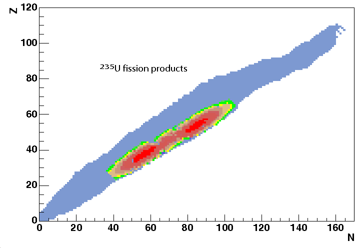
Figure 6.11: Fission yield for 235U. 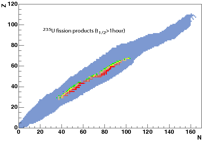
Figure 6.12: Fission yield for 235U with T1∕2 > 1 hour.
6.2.2 Reaction Auto-detection
Reaction auto-detection is based on information found in the ACE binary4 5 format files. Nuclei, for which reaction cross-section database information is available, can be found. The auto-detection process relies on the ReactionList class.
How does it work?
-
First, try to find out if auto-detection has been performed for the given ZAI by reading the binary file “ReactionList/Z.bin” where Z in the proton number of the ZAI. This file contains an array of Boolean for each reaction.
-
If ZAI is not found in “ReactionList/Z.bin”, start auto-detection:
-
Try to find in BaseSummary.dat file the ZAI (or an isomeric state of the ZAI)
-
If it is found, read the ACE file and, among all reactions found in this file, find those which are significant according to a given threshold (see next paragraph)
-
Allow significant reactions and disable all others in ReactionList and add the ZAI to the “ReactionList/Z.bin” file with its reactions.
-
PLEASE NOTE: if the BaseSummary.dat file is modified (add new nucleus, or new base) or if the threshold used to find significant reactions is changed, THE ReactionList DIRECTORY MUST BE REMOVED. Otherwise, your modifications will not be taken into account.
What are significant reactions?
A quantity Ξi is calculated as
where i stands for reaction i. Then if and only if Ξi ≥ σmin where σmin is a minimum threshold, the reaction is take into account ; The default threshold has been set to 0.01 barn6. This can be modified by MURE::SetReactionThreshold() called before any MURE::SetReactionListInitMethod() or Material definition. In order to save time, the procedure to allow or disable a reaction for a given nucleus is performed only the first time an evolution for that nucleus is asked ; then the result for that nucleus (i.e., a ReactionList object) is stored in a file (one per Z) in a specific local directory named ReactionList.
NOTE Any change of the MURE::SetReactionListInitMethod() or MURE::SetReactionThreshold() after a first run will be taken into account only if the nucleus has not been already processed: thus you must destroy the ReactionList directory in order to have these changes taken into account.
6.2.3 The recursion depth cut
It is possible to put a limit on the recursion depth of the reactions when calling the NucleiTree::ExtractZAI method. For example prohibiting 30 or more successive neutron captures limits the nuclei included in the tree to the top of the actinide region (e.g Fermium, Californium, etc.) where experimental cross-section information does not exist, and many successive neutron captures are the only way in which these nuclei can be produced. The recursion depth parameter should be used with care. Figure 6.13 shows the effect of the recursion depth. The default value is 10000...
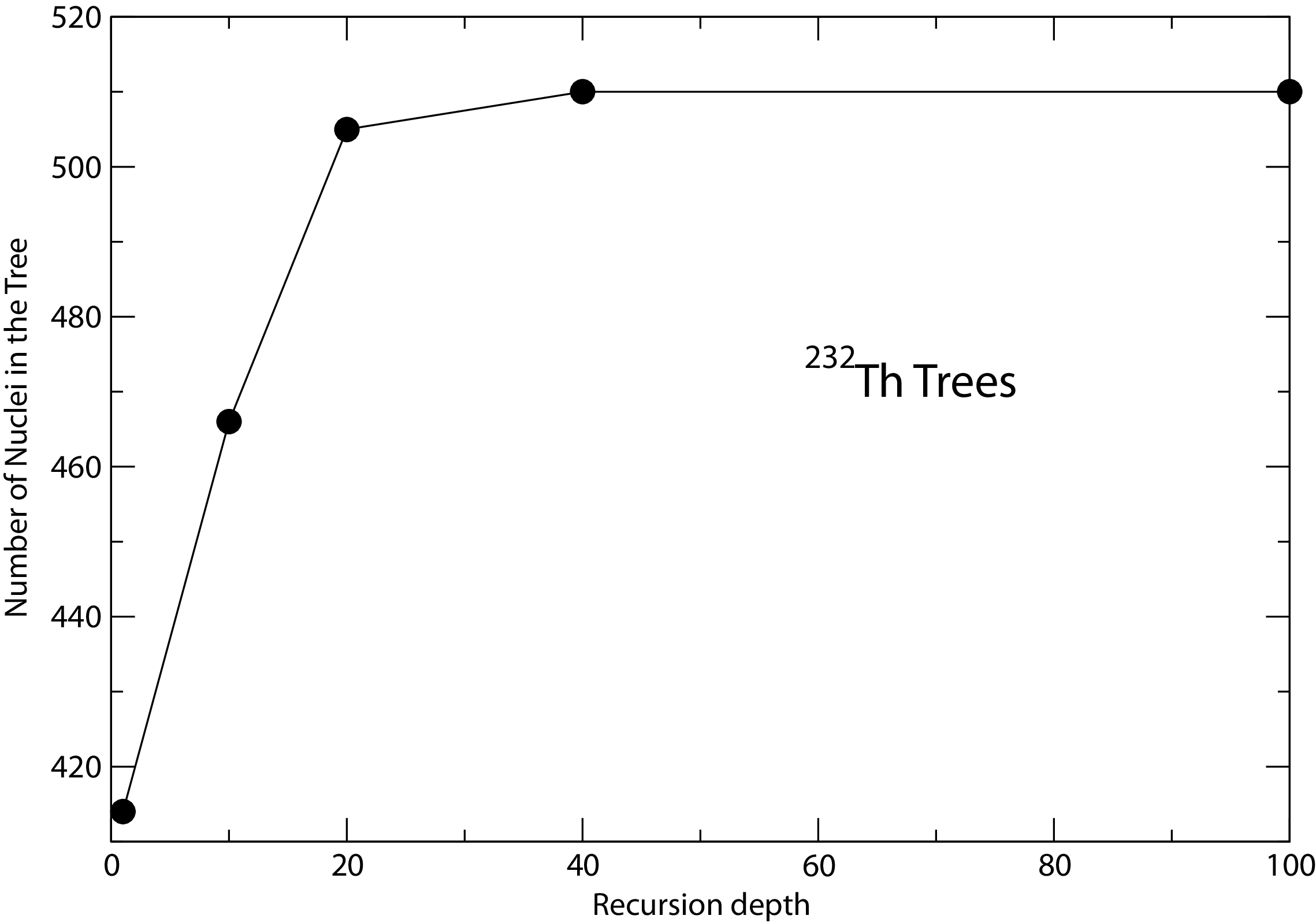
Chapter 7
Evolution in MURE
7.1 Preliminary Remark
Before doing any evolution you must provide a system (geometry based on Cells, all Materials, running MC code mode (critical or subcritical), ...). This system definition is normally provided by the MURE geometry input file (a C++ code). But if you have a very large MCNP file already defined, it is possible to perform an evolution using this file without redefining the whole MCNP geometry in MURE style. The way of doing this is explained in section 7.5. This has not been yet implemented for Serpent.
7.2 General Considerations
Simulating time evolution involves solving the well-known Bateman equations for every given nucleus in every given cell for which evolution is desired, and carrying out this integration over a discrete number of time steps. Simulating the fuel burn-up may also involve adjusting the neutron flux value at every step of the integration process so as to model constant reactor power, adjusting poison concentration to keep a given value for keff, ...
Implementation of evolution related methods are handle via the EvolutionSolver class. An object of that class is automatically built in MURE constructor, thus on can access to it via gMURE->GetEvolutionSolver().
The general scheme for the evolution is shown in figure 7.1:
-
The nuclei tree is built once and for all at the first MC run ; it is controlled via the Material::SetEvolution() method which must be called for each evolving Material before any cell definitions are made. Initial compositions of all materials are entered by the user and these will evolve automatically.
-
All the necessary tallies for calculating mean neutron fluxes and cross-sections in evolving cells are automatically built.
-
The MC input file with the composition at a given time ti is built and a MC run is performed.
-
Bateman equations are solved for (CRAM or Runge-Kutta method) using fluxes and cross-sections of the MC run over a given Δti
-
A new MC file with the composition at ti+1 = ti + Δti is built, and so on.
At the present time:
-
User must provide all ti in a vector of double where the ith element is the value of instant ti at which the Monte-Carlo transport is to be performed.
-
EvolutionControl is used to define evolution conditions (constant power, keff adjustments, ...). Using inheritance, you may develop your own EvolutionControl class (see for example the PoisonEvolutionControl class and § 7.4).
The results of an evolution consist of a number of files stored in an “evolution” directory ; the name of this directory should be defined by the user via the MURE::SetMCRunDirectory function. Two general sorts of files can be found in this directory : On the one hand, there are the MC input and output files (“o”, “m”, “s” and so on for MCNP and “_res.m”, “_det0.m”, ... for Serpent) and on the other, the MURE-generated summary files (DATA_i, BDATA_i, ...) that can be read by a ROOT (see ROOT home page) C++ interface: MureGui.
7.2.1 Time discretization
There are 2 or 3 levels of time discretization:
-
The first level is the MC step, i.e., the number of Δti or MC runs. These steps are user-defined and may be irregular.
-
The second level is the discretization within a Δti. Each Δti is divided in Nsubsteps equally spaced for CRAM or Runge-Kutta δt steps (which we’ll also refer to as evolution sub-steps). At each tk = kδt, Bateman equations are built with given cross-sections. Special methods controlling the evolution could be called at these times (e.g. the flux is renormalized to keep the constant power, ...).
-
Then the last discretization step is performed automatically by the adaptive step size RK method. During this step (discretization of δt in dtrk) cross-sections as well as fluxes are kept constant. Of Course this discretization only applies for Runge-Kutta integration.
7.2.2 The Bateman’s Equation
Here is the general form of the first-order differential equation that has to be solved for every nucleus in every evolving cell.
In the decay part, the meaning of j → i is that the sum of j is done only for nuclei j that decay to i ; in the production of the reaction part, the branching ratio is 0 if the reaction r on j does not produced i, 1 in most of production reaction, except for fission where Rj→i is the fission yields of nucleus i associated to the fission of j, or when reaction produced an isomer and a fundamental state of a nucleus, then it is the production branching ratio of the wanted state (in a evolution, isomer and fundamental are considered as 2 different nuclei).
The writing and solving of these equations are systematically carried out by using internal methods of the EvolutiveSystem class. Only the general approach will be specified here. This approach involves the definition of what is called the evolution matrix E for every evolving cell. The user does not need to know in detail how it works and it is only being described here for the record.
7.2.2.1 The evolution matrix
Internally, every evolving cell knows which nuclei it contains (initially) or will eventually contain due to the evolution of its initial composition, thanks to the prior construction of the nuclei tree (c.f. NucleiTree in chapter 6). The approach taken in MURE is to assign unique indexes to every nucleus in the cell’s composition so as to build its evolution matrix E. It is a square matrix of n dimensions, n being the total number of nuclei in the composition of the cell.
After completion of the matrix, the ith nucleus of a given cell will evolve according to its own Bateman’s equation which will then be simply written as the sum over all nuclei:
where Eij is the corresponding element of matrix E and represents the contribution of the jth nucleus in the cell’s composition to the rate of change in time of the ith nucleus.
The actual writing of the matrix follows the natural structure of Bateman’s equations and is done in two separate parts : first by taking into account all parent/daughter decay relations between nuclei considering proper decay branching ratios. After this, the parent/reaction daughters term is added, where, in the case of fission, fission yields are properly considered.
The evolution matrix is rebuilt in this way at every CRAM/Runge-Kutta sub-steps (c.f : 7.2.1 Time Discretization) for all evolving cells. The solving for the material’s composition new proportion vector  = {N 0, N1 ,…,Nn} is done automatically using either a CRAM or a fourth-order Runge-Kutta-type integration method.
7.2.2.2 Multi-Threading parallelization
Since gcc version 4.1, OpenMp multi-threading is available with gcc compilation. Depending on the distribution, libgomp library (omp.h and libgomp) need to be installed.
The multi-threading behavior is controlled by the OMP_NUM_THREADS environment variable. Setting it to 1 is equivalent to the single processor mode. Setting it to the maximum number of cores available, will run on all that cores (which is the default when this variable is not set). This variable only controls the behavior of the evolution NOT the MC run itself (which is still controlled by the MURE::SetOMP() method).
7.2.2.3 Cooling period
Whereas in general the evolution is useful when the reactor runs at its given power, it is also possible to introduce some cooling period, where the power (and thus the flux) is set to 0. This is done by using an array of booleans of same size than the time vector at which MC runs are normally performed. Each time this array contains a “true”, the flux is imposed to 0 for the considered step, else the evolution is a standard one. The array is passed to MURE via gMURE->GetEvolutionSolver()->SetCooling() method.
7.2.3 Solution of the Bateman equation
The numerical solution of the first order differential Bateman equations is subject to research for a long time. Since the half-lives vary from some seconds to million of years the stiffness of the equation system is challenging for any solution strategy. The most famous and widely used solution of the last century was the algorithm of the ORIGEN [28, 29] code. The nuclei are subdivided into short- and long-living. The first ones are brought into saturation, the latter are solved for by the Taylor series expansion. This numerical scheme is fast, but has shown shortcomings in accuracy.
As already said, in MURE, two methods are actually available to solve Bateman’s equations : a 4th order Runge-Kutta method and the Chebyshev Rational Approximation Method (CRAM) which is now the default. These equations are integrated between 2 MC steps. The EvolutionControl class allows us to interact with the evolution via some methods (just after a MC run, during the evolution, just before the new MC run, see EvolutionControl class). Interactions could be done at each sub-step via EvolutionControl::ControlBeforeEachSubStep. This implies to provide the number of sub-steps in between 2 MC runs which is done via EvolutionSolver::SetNSubSteps (default is 10) or via EvolutionSolver::SetSubDT (in this case, a δt is provided, and the number of sub-steps is calculated accordingly).
7.2.3.1 4th order Runge-Kutta
The fourth-order Runge-Kutta method is a very well-known and standard method to integrate ODE ; it is generally a good compromise between speed and accuracy compare to higher (or lower) order. The method implement in MURE is adapted from Numerical Recipes[30] and is coupled to an adaptive step size. To use it:
-
gMURE->GetEvolutionSolver()->SetDepletionSolver("RungeKutta");
7.2.3.2 Chebyshev Rational Approximation Method (CRAM)
A quite elegant and accurate solution called CRAM was recently developed by M. Pusa[31, 32, 33] and has become kind of a standard solution to Bateman equations in nuclear systems. The method is very effective for matrix systems where the eigenvalues are distributed near the negative real axis. Several formulations for CRAM exist. Because of better numerical stability the method of incomplete partial fractions (IPF) is adapted with orders from N=4 up to N=48 and the CRAM coefficients are taken from the publication[33]. The IPF algorithm foresees a series of N/2 matrix inversions, which are of type sparse matrix because of the nature of the burn-up (transmutation) matrix. The matrix inversion can be done by a Gauss-Seidel iteration or – in this case – by the solver SparseLU of the Eigen library[20].
Dependent on the time range of the half-lives the recommended order lays between 16 and 48. If not requested a specific order the code chooses the suitable order for a given matrix system and time-step. CRAM has become the default solver of MURE[34]. Its options may be addressed by following methods:
-
gMURE->GetEvolutionSolver()->SetDepletionSolver("CRAM"); // default
// setting explicitly the order deactivates the search for the lowest suitable order
gMURE->GetEvolutionSolver()->SetCRAMOrder(48);
gMURE->GetEvolutionSolver()->SetCRAMMethod("IPF"); // only IPF available (default)
In MURE v2 the sparse solver was based on the Eigen::SparseLU solver which shows deteriorated performance the larger the time interval becomes (in the order of 30 days). The default solver now is the Eigen internal BiCGSTAB solver. However, one may choose an UMFPACK [35] accelerated external solver of Eigen from SuiteSparse1 which could be even more powerful but it is very system dependent due to interaction of BLAS/LAPACK with pThread or OpenMP2.
7.3 Different way of evolution
We suppose that the evolution is done at a constant power. Evolution can be performed in different ways that can influence the result.
-
Evolution with a “constant” reaction rate: this is the default. Between 2 MC steps, reaction rates are keep “constant” ; a new reaction rate evaluation is performed at the next MC run for the next step. In fact, they are not really constant: due to renormalization of the flux to keep constant power, reaction rates used in Bateman equations are in fact, ασϕ where α is the flux renormalization coefficient. Thus, periodically within a MC step, these reaction rates are readjusted (this explains the use of the term “constant” in quotes). An example of such evolution can be found in MURE/examples/Depletion/EvolvingSphere.cxx or MURE/examples/Depletion/EvolvingSphere_serpent.cxx
-
Cross-section evolution: this is no longer the default. Previous MC runs are used to linearly extrapolate the reaction rates for the next step.
-
Window average evolution: a mean (σϕ) is calculated from the previous MC runs and the actual one ; this mean value is used to solve Bateman’s equations. The window to compute average is based on EvolutionSolver::GetFitRangeNumber() previous runs (default is 4).
-
Predictor-corrector methods. TO BE NOTICED: Because no real advantage of this methods have been found, this way of evolution is not more maintained. So new MURE (from MURE v2 alias SMURE) development have probably broken this way of evolution which is discouraged. There are 3 Predictor-corrector (PC) methods implemented. This is actually new and not fully tested (despite the fact that it currently works). Suppose that the MC run at time TN has been done (leading to reaction rates (σϕ)N). The evolution has to be performed up to TN+1.
-
PC at middle point: the predictor run is performed with “constant” reaction rates (σϕ)N up to TC =
 ; then a corrector MC run is performed and leads to (σϕ)C. Starting with the composition of TN, the evolution is done again from TN to TN+1 with the “constant” reaction rates (σϕ)C evaluated at the middle point.
 -
PC at end-point: the predictor run is performed with “constant” reaction rates (σϕ)N up to TC = TN+1 leading a composition CN+1P; then a corrector MC run is performed and leads to (σϕ)N+1. Starting with the composition of TN, the evolution is done again from TN to TN+1 with the “constant” reaction rates (σϕ)N+1 leading to a composition CN+1C. Then, the composition used for the next predictor run (for TN+1 to TN+2) is CN+1 =
 .
. -
Kind of PC at end-point: the predictor run is done like in b) but for the corrector run, we used a linear interpolation of reaction rates from (σϕ)N to (σϕ)N+1. The next composition for TN+1 to TN+2 is CN+1 = CN+1C.
First tests seem to give an advantage to method b) for the quality of its results (compositions, dispersion of composition for M identical run with different random seeds, ...).
-
-
Multi-Group evolution[11]. If this method is used, not that reaction rate tallies are not built in the MC input file ; instead, a thin energy binning flux will be built for each evolving cell. Then, after the MC run, reaction rates are calculated as ∫ ϕ(E)σr,i(E)dE where the sum is done over each energy group, σr,i is the pointwise cross-section of reaction r for nucleus i read in the ACE file used for MC run (if ASCII version is used, please note that this will take longer...). The main advantage of this method is a considerable CPU time saving (more than 30 times faster3 than the “standard” evolution). The accuracy of the result are quite good (~1% for thermal systems and 5% for fast ones4). To use this method, one has to define “gMURE->GetEvolutionSolver()->UseMultiGroupTallies();” at the beginning of the input file (see MURE/examples/Depletion/EvolvingSphere2.cxx example). The default energy binning for flux is (72995 groups)
Energy range 10−4eV - 1eV 1eV - 10eV 10eV - 10keV 10keV - 0.1MeV 0.1MeV - 20MeV Number of bins/decade 2000 2000 5000 2000 1000
The main problem of multi-group evolution is the 238U. Its capture cross section has been chosen to “optimize” the group structure (number of bins/energy interval). In order to take the advantage of the multi-group CPU time saving, it has been implemented the possibility to use multi-group runs for all nuclei but 238U : in that case, the “standard” method (real MC tally) is used for 238U, and multi-group tallies for the other nuclei. This is done by setting the “StdTallyFor238U” to “true” in the “EvolutionSolver::UseMultiGroupTallies()” method.
7.3.1 Cross-section Evolution
Cross-sections are evolving with time because of the flux shape evolution. Between 2 MCNP steps, cross-sections are either constant, either evolving. Taking the cross-section evolution during the “evolving step” should enable a better precision and increase evolution step duration, reducing the CPU time. It is based on linear extrapolation of previous MC runs.
!!!! After a study of error propagation, it appears that fitting σϕ leads to a bigger dispersion of cross-section evolution in the result (with a constant power). Thus this treatment is no more used by default. To use it you must specify it by a MURE::FitSigmaPhi(true).
7.3.1.1 How does it work?
The treatment is applied for each cross-section of each nucleus in each cell. Thus, for the sake of simplicity, we will only consider a reaction cross-section σi of a nucleus in a cell.
Since for evolution, reaction rates are used, we should rather consider the reaction rate σiϕ and not the cross-section σi. Suppose that we have performed an evolution up to step k (i.e., kth MC run is just finished). To know the reaction rate evolution up to step k + 1 (i.e., just before a new MC run), a linear fit (least square method from Numerical Recipes) is applied to EvolutionSolver::GetFitRangeNumber() previous MC reaction rates5 (that is to say, MC runs k − 3, k − 2, k − 1, and k). Then, for the evolution over step k → k + 1, the reaction rate is extrapolated with (σiϕ)(t) = at + b, where a and b are the results of the linear regression. Note that for the first EvolutionSolver::GetFitRangeNumber() MC runs, reaction rates are kept constant.
As already mentioned, integration of Bateman equations is in fact done in N sub-steps by either the CRAM method or by a 4th order Runge-Kutta steps which are automatically divided in other shorter time steps (adaptive step RK method) ; the reaction rate evolution is only performed at each sub-step level and it is kept constant within the current sub-step. This constant value is evaluated in the middle of the sub- step to be more accurate (see fig. 7.2).
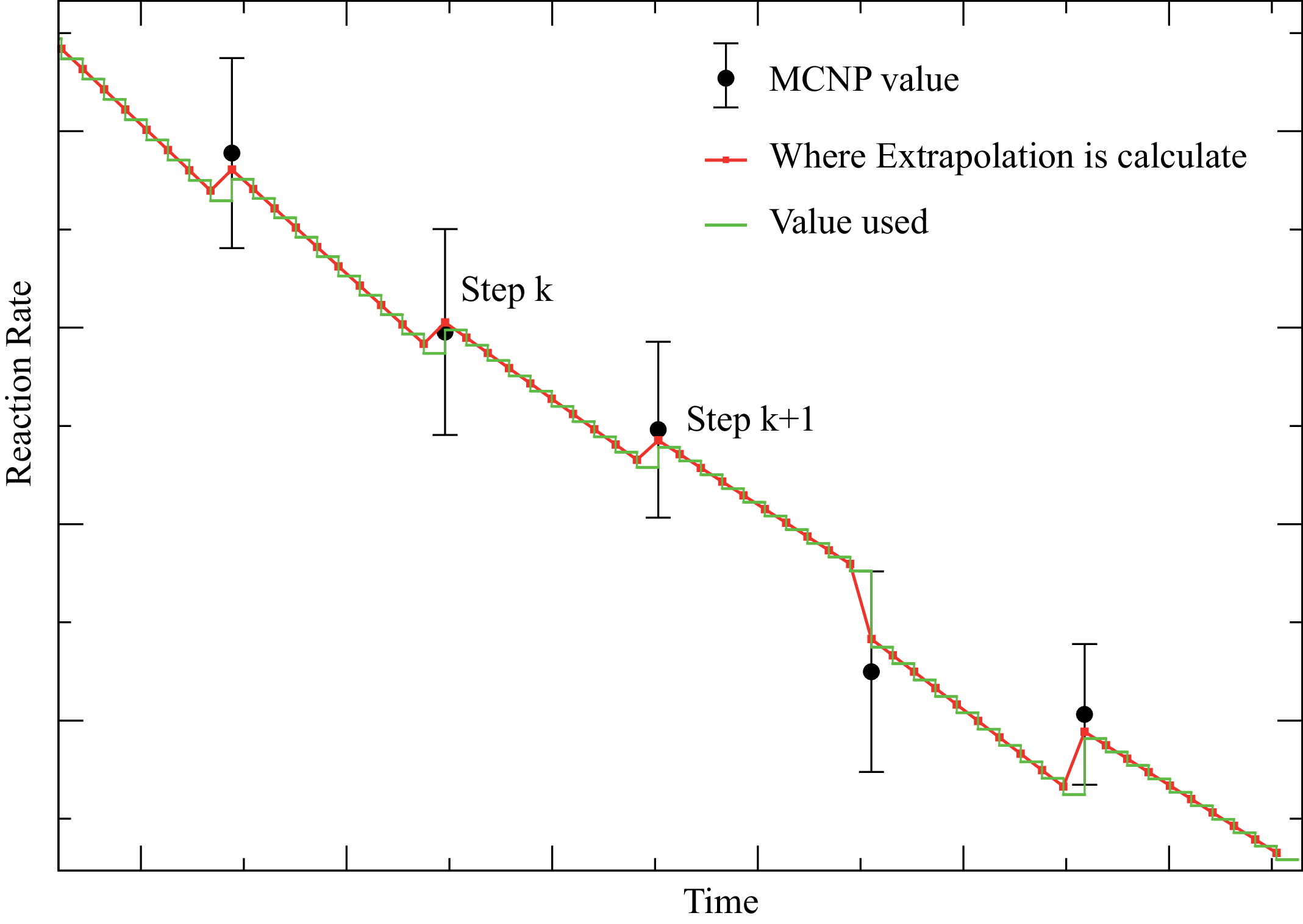
In order to better consider the rapid variation of a reaction rate slope, we have slightly improved the method as follows (here Nfit =EvoltionSolver:: GetFitRangeNumber()) :
-
a linear regression is performed on Nfit to obtain a′ and b′ for the reaction rate evolution
-
a linear regression is performed on Nfit − 1 to obtain a′′ and b′′
-
then if the 2 slopes a′ and a′′ are of opposite sign, the slope taken for the evolution is the mean a =
 and b =
-
or else, a = a′ and b = b′ if |a′| < |a′′| or a = a′′and b = b′′ if |a′′| < |a′|
7.4 Reactivity Control
NOTE: only few tests have been performed and therefore many bugs may be present in the Evolution Control.
As already mentioned, the control of the whole evolution is done via the EvolutionControl class. This class already includes some useful methods, but the best thing to do in order to implement your own control is to write a derived class. In a first example, the reactivity control uses the original EvolutionControl class ; then the way of implementing your own control will be given. The EvolutionControl class inheritance tree is shown on Fig. .7.3

7.4.1 A simple example using standard EvolutionControl
The example file poison.cxx (MURE/example/poison.cxx) corresponds to a very simple reactor (cylinder of borated water with a hexahedral fuel pin lattice). The reactivity control is done by adjusting the concentration of a poison (the boron) in the water. We assume that a large reserve of boron is available and thus, when necessary, we can adjust the boron concentration at a desired value. The method principle is to calculate an estimation of keff using the reaction rate extrapolations:

(n,xn), “escape” and σpoison are supposed to be constant between 2 MC steps ; the poison concentration Np is thus determined using the desired keff in the formula.
7.4.1.1 Poison material declaration
-
ControlMaterial *BoratedWtr=new Material (0.7187023, 673);
BoratedWtr->SetDensity(0.719);
BoratedWtr->AddTheControlNucleus(5, 10,0.00012);
BoratedWtr->AddTheControlNucleus(5,11,0.00048);
BoratedWtr->AddNucleus(8,16,0.333);
BoratedWtr->AddNucleus(1,1,0.667, "H2O");
A ControlMaterial is a Material which is used to control the evolution, and in this case, a poison to control the reactivity. The 3th an 4th lines informs us that boron 10 (and 11) are the nuclei used to control the reactivity. See the “poison.cxx” example.
This material must not be an evolving material, because we’ll consider that we can adjust boron concentration every time .
7.4.1.2 Escape calculation
In the keff formula, neutron leakage is needed ; in order to calculate these escapes, one has to define a F1 tally (current through surface) through the most outer Shape of the geometry ; in the example this leads to:
-
gMURE->SetOutermostShape(Vessel);
because “Vessel” is the outer cylinder of this “reactor”.
7.4.1.3 Evolution definition
You have to declare the Evolution Control object:
-
PoisonEvolutionControl *ECon=new PoisonEvolutionControl();
ECon->AddReactions(BoratedWtr);
gMURE->SetEvolutionControl(ECon);
The 2nd line gives the specific EvolutionControl command to add the required reactions useful for the control (poison absorption, ...)
7.4.2 Using your own EvolutionControl
The aim of this section is to help user implement its own EvolutionControl using inheritance mechanism. Then you will be able to write your own specific methods that will be called for the evolution control. Supposed we wish to create a MyEvolutionControl class: the hxx and cxx files are in MURE/example/.
NOTE: Don’t forget to redefine the EvolutionControl* Clone() as:
-
EvolutionControl* Clone(){return new MyEvolutionControl(*this);}
Each method and variable of EvolutionControl are known in MyEvolutionControl ; but because of the virtuality of some methods, the ControlAfterEachMCRun(), ControlBeforeEachSubStep() and ControlAfterEachEvolutionStep() methods of MyEvolutionControl will be called instead of the ones of EvolutionControl. This means that these original methods of EvolutionControl are no more called, and thus you have to read them carefully to implement what is needed or necessary for your evolution control.
Now to use this new class in Myprog.cxx:
-
#include <iostream>
#include <cmath>
using namespace std;
#include "MureHeaders.hxx"
#include "MyEvolutionControl.hxx"
...
int main(int argc, char** argv)
{
...
MyEvolutionControl *NewEC=new MyEvolutionControl();
gMURE->SetEvolutionControl(NewEC);
}
and to compile one should do
-
g++ -c MyEvolutionControl.cxx $MURECXXFLAG
g++ -o Myprog Myprog.cxx MyEvolutionControl.o $MURECXXFLAG $MURELIBFLAG
where the variable MURECXXFLAG and MURELIBFLAG have been set to (bash example):
-
export MURE_DIR="/path_2_MURE_install_dir/"
export MURECXXFLAG="-g -fPIC -std=c++14 -I$MURE_DIR/source/include -I$MURE_DIR/source/external -I$MURE_DIR/source/thirdparty/eigen"
export MURELIBFLAG="-L$MURE_DIR/lib -lMURE -lvalerr -lmctal"
7.5 Evolution of a MCNP user defined geometry
This section is devoted to users who have already defined a complex MCNP file and would rather not use the MURE geometry capability when making evolution. Even if this task requires some work, the procedure is simple. User has to redefine in MURE style, ALL materials of its geometry and all EVOLVING cells (but not the shapes associated to the cells). Of course, user will need all files required by a standard evolution (BaseSummary.dat, AvailableReactionChart.dat, ...)
The principle is the following: a line by line of a MCNP user input file are copied, but
-
if the cell number found corresponds to one of the “virtual” evolving cells defined, then the density of the evolving material at the given evolution step is taken into account. Be sure that 2 evolving cells must have 2 different materials (because they usually evolve differently even if at the beginning they are the same) ; thus, it is at present not possible to make the evolution of a cell defined by “like but” because there is no material on this cell line.
-
The general MCNP block will be read, but all the material description (“M” and “MT” cards) will be skipped and replaced by the MURE material definition. Note that if one wishes to use source MURE definitions, particle MODE definitions or PRDMP MURE definitions, any “SDEF”, “KSRC”, and “KCODE” (for source) or “MODE” or “PRDMP” must be removed from the original file. If you have defined tallies, they will be copied (line by line) and the necessary tallies for evolution will be constructed starting from your highest tally number : for example, if you defined 2 tallies F34 and F44, the automatic tallies for evolution will start at F54 ; tally numbers 4,14 and 24, are not used.
For material declaration, you must use the special Material constructor that takes as a single argument the material number ; this number is the one you have written in the MCNP input file. Don’t forget to declare ALL materials of the geometry (evolving or non evolving). For non evolving materials, you must ask MURE to include them in the MCNP output file by using Material::AddToGlobalNucleiVector() after the last input nucleus.
For cell declaration, you must use the special Cell constructor ; it takes the cell number (the one you have written in the MCNP input file), an evolving Material pointer and the cell volume (in m3). ONLY evolving cells should be declared.
The Original MCNP input name is defined by MURE::SetUserGeometryInputFile() method. You can also defined all desired cards of the general data block (source, physical card, ...). The rest of the evolution is completely analog to what is explained in the above sections. Don’t forget to provide a mean to calculate the tally normalization factor (you may either give a predefined power or use the MURE::SetTallyNormalizationFactor()).
An example is shown in UserGeo.cxx with the UserMCNPGeo MCNP input file.
7.6 More complex evolution conditions
Sometimes, the evolution is performed with power variations, some parameters such as boron concentration, temperature, ... are changing. This can be achieve through the EvolutionWrapper class (see EvolutionWrapper class) . Such conditions are illustrated on the following example:
-
EvolutionWrapper *EC=new EvolutionWrapper(); // create EvolutionWrapper
EC->AddPhase(100,3,1); // create a new 100 days phase with three MCNP steps, (1=logarithmic discretization)
EC->SetPowerLinear(0,4e4); // raise power from 0 to 40 kW
EC->SetMaterialBoronLinear(Cell_of_BoratedWater->GetMaterial(),1000e-6,500e-6); //boron depletion from 1000 to 500 ppm
EC->AddPhase(100,1,0); // a new single-step 100 days cooling phase
EC->SetPowerCooling();
EC->AddPhase(100,3,0); // a new 100 days phase with three equal(0=linear discretization) MCNP steps
EC->SetPowerConstant(4e4); // power is kept constant at 40kW in that phase
EC->Evolve(); // run the evolution (DO NOT CALL the MURE:Evolution method ; it is done here)
7.7 Equilibrium of Xe-135
In some circumstances, flux oscillations in weak coupled systems creates numerical (unphysical) Xe oscillations. These Xe oscillations enhanced the flux oscillations causing numerical instabilities. To reduce these instabilities, a special treatment has been implemented. To use this treatment, one has to call the EvolutionSolver::SetXe135Equilibrium(double teq) method, where teq is the time from which the treatment is really applied (default time value is 3 × T1∕2135 Xe ∼ 27h).
Here is the description of what is done:
-
if t < teq, then the standard evolution is carried out (i.e. no special treatment)
-
if t ≥ teq, then
-
the 135Xe Bateman equation is imposed to be at equilibrium :
 = 0
= 0 -
the 135Xe is calculated as
(7.1) where yXe is the fission yield for 135Xe, Σfissionϕ is the number of fissions, λi is the decay constant for nuclei i and ϕ is a “mean” flux in the cell calculated as
if there is a factor greater than 1.5 between ϕprevious MCNP run and ϕcurrent MCNP run, else ϕ = ϕcurrent MCNP run
-
the 135I used in (7.1) is calculated in the same way :
but this value is only used in for the (7.1). To be noticed, that in general, due to its very short period (T1∕2 ∼ 19s), the 135Te is absent of the evolution ; it is then taken into account in the iodine fission yield yI as explained in the Nuclei Tree section (c.f. 6).
-
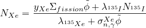
Chapter 8
Looking at results from the evolution
8.1 The MURE data files
At present, results from the evolution are stored in the MC Run directory. There are 4 types of MURE files generated in addition to the MC files for each evolution step:
-
DATA_xxx files are written for each step number xxx, and contain not only the Material composition information, but also average cross-sections for every possible reactions for all evolving cells in the geometry. In addition, average flux for each cell, cell spatial variables (if defined), keff, and time are also written out. They are written just before CRAM/RK sub-steps ONLY IF EvolutionSolver::SetWriteASCIIData() has been called.
-
DATA_xxx.json files are very similar to the DATA_xxx files except that the format is based on the JSON (JavaScript Object Notation) format using the Niels Lohmann’s JSON for Modern C++ library[21, 22]. They are written ONLY IF EvolutionSolver::SetWriteASCIIData() and EvolutionSolver::SetWriteJsonFormat() have been called. To be noticed that this format, by far more readable, produces slightly bigger files (which are thus longer to read).
-
BDATA_xxx files contain the same information as the above files but in binary format. Initially it was expected that these files would be much shorter in length than the ASCII files, but it appears that not much space is saved if binary files are used to store MURE results. Nevertheless it is much faster to use these files for post-treatment. They are written just before CRAM/RK sub-steps by default. On can disable this writing by using EvolutionSolver::SetWriteBinaryData(false).
-
KDATA contains all the keff information (with statistical errors) for all evolution steps in one file. These data are also contained in [B]DATA_xxx.
-
FDATA contains all the data pertaining to the fission rates of various nuclei. For all the 50 or so nuclei which can fission, the rate (in fissions per second) integrated over all the evolving cells, is written out.
When using reprocessing feature DATA_bxxx or/and BDATA_bxxx files are also written just at the end of CRAM/RK sub-steps. When using PoisonEvolutionControl, additional files are also written such as POISON_PROPS which contains the poison proportion as a function of time.
8.2 Reading the data files with Tcl/Tk graphical interface scripts
This graphical interface is now deprecated. Except for ExamTree.tcl
-
ExamTree.tcl
To run these scripts from anywhere it is a good idea to add the TclScripts directory to your path. You must also set the DATADIR environment variable.
-
The ExamTree.tcl script is useful for exploring the evolution nuclear tree, which can be written out for the global nuclei vector of the MURE class using gMURE->WriteAsciiTree(“myfile.dat”); or the tree for a material object Material->DumpTree(“myfile.dat”); To explore the tree, type
ExamTree.tcl myfile.dat
Everything else is intuitive and self-explanatory. Just click either on the nuclear chart, or the Nucleus X window.
8.3 Reading the data files with ROOT graphical interface
This is a C++ GUI base on ROOT. Thus, before using this GUI, you must install a recent ROOT version (5.0 or any later version). This is easy because binary files can be downloaded from the ROOT home page (http://root.cern.ch). We have chosen ROOT because:
-
it provides a large number of widgets
-
it is a very simple way of modifying, saving graphs: zoom on axis, grid, log scale, changing font, color, text position and so on as well as various picture saving formats are available (eps, jpeg, png, gif, ...).
The GUI sources are in MURE/source/gui and the install version is in MURE/mure3/bin ; the best way to build this GUI, is to use the “build.sh --enable-gui” script and to set environment variables in your .basrc accordingly to what the build.sh script proposed. If Lapack package is available, the radiotoxicity analysis will be possible. LAPACK is a Linear Algebra PACKage used to solve the set of coupled differential equations for decays by a matrix diagonalization procedure. If this package is not installed, you have to install it (see § 1.4.4) to run the radiotoxicity module (but all other MureGui capabilities can run without Lapack). The MureGui executable has the following syntaxe:
-
MureGui [-help -h -onlytox -start num -font factor -color] DirName1 [DirName2 ...]
where
-
DirName1 is the MURE evolution directory (containing the BDATA_* or DATA_* files) and optional DirName2, ... are other directories to compare evolution. The line style of plotted graphs is different for each directory (solid=DirName1, dash=DirName2, dot=DirName3, dash_dot=DirName4, ...). NOTE: when comparing evolution, you must be sure that the cell composition of the different evolution are the same: the list of non empty proportion nucleus must be in the same order.
-
-onlytox : this flag allows to study the out-of-flux decay of nuclei ; a detail description is done in §8.3.6.1
-
-font factor: factor is an integer (>0 or <0) to increased the font size of widget. Default: 2 ; Try +/- 2 before adjusting.
-
-color : by default if the number of cross-section or reaction rates are big, the color is suppressed for these 2 tab of MureGui ; if this flag is used, this forced the color used but it is VERY SLOW.
-
see MureGui -h or -help for a complete explanation of options.
A module in the transport code DRAGON has been developed to copy the results in DATA ASCII file format.
The interface has a Main windows composed of 8 tabs (Inventories, Cross-sections, Fluxes, Reaction Rates, K_effective, Breeding Ratio, Radiotoxicity and Spatial Variables, see Fig. 8.1
) and can have up to 8 plot windows (one for each tab).
Whereas MureGui is graphical interface, the “Terminal” window used to run this program is often used for some important warnings/information/output: don’t forget to look at it!
8.3.1 The 8 tabs of the main window
-
In the Inventory Tab, colors of nuclei (see Fig. 8.1) correspond to the total mass scale importance (red: large mass->black: small mass). Nuclei are sorted in 4 categories (Actinides, Fission Products, Gas, and Miscellaneous) but a nucleus could belong to more than one category (a gaseous fission product is in FP and in Gas). “FP” and “AM” check boxes allows respectively the plotting of total fission products and total minor actinides (Np and Am, Cm, ...) . The total mass of checked nuclei can also be automatically performed using the “Sum of Selected” check boxes1. Finally, nuclei inventories are given in “Mol”, “Mass(g)”, “Mass/ton(kg)”, “Density(At/(barn.cm)” or “%At. Selected”. This last quantity is the number of atoms of a given selected nuclei divided by the sum of atoms of all selected nuclei ; this allows for example to plot the plutonium vector at each evolution step. The “mass/ton” radio-button normalizes the plotted mass (in kg) by the ton of initial heavy nuclei. When several physical cells i are selected (see later with Spatial Variable combo box), the total inventory of one nucleus is simply given by the sum of inventories in each region. Thus we have:

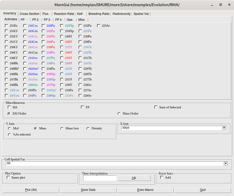
-
In the Cross-section Tab, colors only help users to see the isotopes (all reactions for a same isotope are on the same color). The “FP”’ check box allows the plotting of the mean fission products total cross-section. Similarly with the Inventory tab, the total cross-section can be obtained with the “Sum of Selected” check box (but FP and AM check boxes are not taken into account in the sum). Microscopic and macroscopic cross-sections are available. When several physical cells i are selected (see later with Spatial Variable combo box), an equivalent cross-section Σ is computed for all reactions to maintain their total reaction rate:
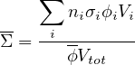
where the nuclei density is ni =
 , the mean flux is ϕ =
  and the total volume of all cells is V tot
= ∑ iV i. The numerator is the total number of reactions in all i-cells. Thus, one can define an equivalent microscopic cross-section:
and the total volume of all cells is V tot
= ∑ iV i. The numerator is the total number of reactions in all i-cells. Thus, one can define an equivalent microscopic cross-section: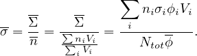
Note:-
when the density of one nuclei is null, a very small and uniform density is used to compute the equivalent microscopic cross-section (n = 10−20at.cm−3).
-
This mean cross-section is useful to compute “simplified” Bateman equations. But one has to be very attentive to its physical signification when lot of cells with different fluxes and concentrations are involved ; then this mean value may be greater than all individual cross-section of each cell due to an under estimation of the denominator.
-
Sometimes, it may be useful to compute the mean microscopic cross-section over the spectrum:
Then one can compute a average cross-section over the cells as ⟨σ⟩ =
 . In MureGui, one can plot this kind of microscopic cross-section by selecting the “Micro (spectrum)” radio widget.
-
-
In the Flux Tab, the “All cell” and “Sum of Selected” check boxes allow users to plot a mean flux over all or selected evolving cells i. The mean flux is given by:
-
In the Reaction Rate Tab, the “FP” and “Sum of Selected” check boxes allow users to plot total reaction rate of fission products and the sum of selected reaction rates respectively. The generated power can also be obtained using the “Power” check box. Power results are returned in the terminal when the graph is refreshed. The “(Un)Select Fissil” button selects (or unselects) all available fission reactions automatically. Note that released energy per fission values (Q_values) are automatically selected according to the transport code previously used (DRAGON, MCNP or Serpent). In this Tab, it is also possible to plot Neutron Balance normalized per 1000 fissions. Once the user has selected the wanted reaction rates (or all reaction rates for the fissile (“(Un)Select Fissile” button) or for all nuclei (“(Un)Select All” button), the neutron balance is plotted using histogram bars. The box “Threshold to Others” allow user to group all reaction rates less than the threshold (default 0.1 per mil) in a category named “Others” (see fig. 8.2 and fig 8.3). The “Dir” number is the number of the Dirname argument of MureGui and the number following the “@” character corresponds to the time at which the MC run is done (thus figure 8.2 corresponds to first Dirname at time t=1004.44 days where a MCNP run was performed)
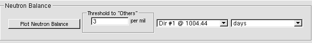
Figure 8.2: Neutron Balance window. In this example, the reaction rates less than 3 per mil are grouped in the “Others” category. 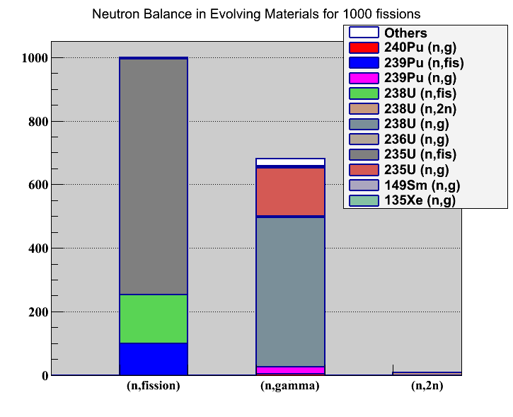
Figure 8.3: Neutron balance plot. -
In the Keff Tab, the “Keff ” check box allows user to plot the multiplication factor keff of the assembly with evolution time. The “Average Keff ” check box computes and plots the average neutron multiplication factor keff of an assembly along its life. It is particularly useful in CANDU reactors at the refueling equilibrium state. The average value keff is given by:
-
In the Breeding Ratio Tab, users have to select some nuclei among all heavy elements in order to define them as fissile for the calculation of Breeding Ratio (BR) and Fissile Inventory Ratio (FIR). The (instantaneous) BR is computed at a given time t as the ratio of the total production rate of the so-defined fissile nuclei at time t over the total disappearance rate of the same nuclei at the same time. Up to now, only fissile nuclei among 233U, 235U, 239Pu and 241Pu can be defined as fissile and taken into account for BR calculation, with a special treatment for 233U (which production rate is 233Pa decay rate) and 241Pu (which disappearance rate includes its decay rate).
The FIR is computed as the ratio of fissile nuclei between actual and initial time :
Note that if the initial fissile nuclei mass is 0, no plot is returned. In the case of 233U selected as fissile, selecting 233Pa as fissile too gives access to the effective FIR values, with each calculation time as a possible End Of Cycle. Indeed this accounts for 233Pa out-of-flux decay, producing 233U without loss. In this case, a warning is printed to inform the user that 233Pa is used this way only for FIR (BR is still computed without Pa-233 defined as fissile, and using its decay rate as 233U production rate).
-
In the Radiotoxicity Tab (see also section 8.3.6), shown in Fig. 8.4, (only if Lapack library has been found), decay calculations can be performed for the final inventory after an evolution has been done. Determination of total and partial radiotoxocities, heat released and activities as a function of time can be computed for a given system. Note that if, for radiotoxicity post-treatment, MureGui is used from in a directory where the MURE “data” directory is not present just above the current path, you must define the DATADIR variable (using the standard environment variables: export DATADIR=”$MURE_DIR/share/data”).
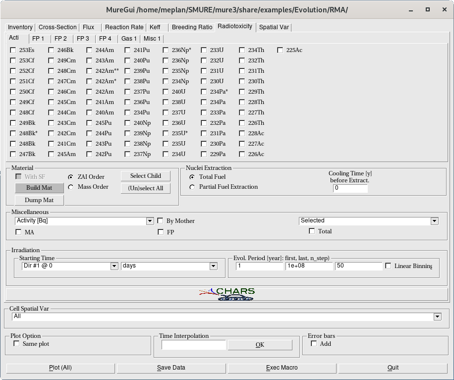
Figure 8.4: MureGui : the radiotoxicity Tab. -
Users should click on the red “Build Mat” button before taking any further action. This will compute the Material and the matrices. The material is based on the material defined in the DATA or BDATA files where all the nuclei are copied, and all their decay children. No cut-off is used to select the children. By default, spontaneous fissions are not taken into account ; in order to allow it, check the “with SF” button BEFORE clicking the “Built Mat” button. The matrices for decay calculations A are also computed once and for all. The variation of the isotopic vector N is given by:
where tc represents the cooling time (after irradiation). The solution of this equation is simply given by:

This equation represents a set of coupled differential equations for the decays which is solved by a matrix diagonalization procedure based on the LAPACK standard libraries (resolution is performed at the beginning). Inventory composition over time is then directly obtained from the initial composition.
-
The “Nuclei Extraction” frame allows user to specify what percentage of nuclei of the current composition is taken into account for activity, radiotoxicity, ... calculation. When one choose “Partial fuel extraction” a new window appears to choose the per cent of category you keep: 100% means that all that category is kept. For example, putting 100% for all categories except 1% for U and Pu mean that the radiotoxicity is calculated for the initial composition where only 1% of the U and Pu nuclei are kept, all other nuclei being completely taken into account. User can choose a cooling time before the extraction occurs. In that case, the plot window will start for t = 0 after the core discharge to the cooling time value2 ; then, the partial extraction is done and the result is plotted. A dash red line is drawn to show the time of extraction. A “Chars” logo button allows user to plot energy spectra of γ, β, α and neutron emission of “spent fuel” (see section 8.3.6).
-
In the “Miscellaneous” frame, one can also select the value to be plotted: “Activity”, “Radiotoxicity”, “Heat” released and “Inventory”. By selecting the “By mother” check button, the radiotoxicity is computed by mother nucleus (i.e. present at the starting time) in order to see the contribution to the activity of a given nuclei (the daughters of this nucleus are part of its activity). Note, the “By mother” calculation takes much more CPU time! ”FP”, “MA” and “Total” check boxes allow one to plot the total value for fission products, minor actinides, and all nuclei respectively. A combo box can be used to plot “selected” nuclei, “selected nuclei & their sum” or “only the sum” of selected nuclei (FP and MA check boxes are not taken into account in the sum).
-
In the “Irradiation” frame, see Fig 8.5, one can choose the burn-up of the spent fuel (i.e., the MCNP step given at a time). The “Dir # num” allows to choose which evolution directory to consider in the case or more than one evolution directory is given to MurGui arguments. The evolution (cooling) of the spent fuel is specified by the evolution parameter: the cooling starts at t = 0, but the plot start at the first value of the “Evolution Period” frame ; the final time, number of time-steps and whether the steps are logarithmic or linear are then given. Note that the graph are on a log scale, thus, initial time has to be strictly positive (minimum value is 1 minute). The number of steps does not affect the results, but only the smoothness of the curve.
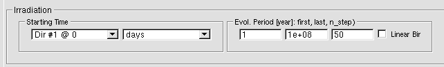
Figure 8.5: “Irradiation” frame. Here, the first Dirname at time t=0, i.e., the first MCNP step, is used. The fuel cooling will be plotted from 1 year to 100 million of years with 50 log steps.
-
-
The “Spatial Var” tab allows the plotting of spatial flux (or power deposit) dependence if you have defined spatial variables (see the Cell class and next paragraph). It is present only if Spatial variables have been defined. The “Plotting Time” frame allows user to select the time at which the plot is done. The “Variable choice” frame allows user to select what to plot (in the “Plotting Variable” combo box) and with, eventually, a condition on spatial variables (“Conditional Variable” combo box). For example, if a core has been divided in N radial zone and M axial zone, you can plot the mean flux as a function of Z for every radial zone (see figure 8.6). One can also plot this flux but only for a given radial zone by selecting the desired “ring” in the “Conditional Variable” combo box. The “Same Plot” check button, allow users to overlap plots.
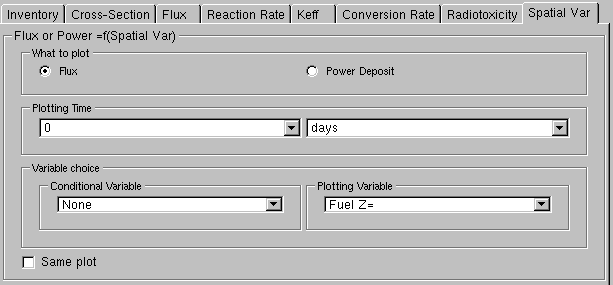
Figure 8.6: Spatial Var Tab - This will plot the flux as a function of Z for t = 0 whatever the spatial variables (no condition).
8.3.2 Frame “Cell Spatial Var” in the Main window
Users can define Spatial variables for cells (see the Cell class). The aim of these variables is only to extract results in a simpler way (this means that you can add spatial variables after the evolution is done and redo the evolution keeping MCNP files without any problems). If such variables have been defined you can plot quantities according to spatial variables.
Suppose we have done the evolution of 3 rings of a cylindrical core divided in 3 parts along the cylinder axis. If, for each of these 9 evolving cells, 2 spatial variables named “R” and “Z” with value corresponding to the typical cell locations have been defined, then the combo box of the “Cell Spatial Var” will allow users to plot for example 235U quantity for all cells with a particular radius Ri (i.e. whatever other Z value, see Fig 8.7) or to plot this quantity only for a given Ri and Zi (see Fig 8.8)


8.3.3 Frame “Time Interpolation” in the main window
A linear interpolation is performed on the plotted data for the selected Tab at the corresponding time (and not the selected data of this Tab). Results are returned in the terminal. Note that no time unit is specified, thus it must be coherent with the plotted data.

8.3.4 Frame “Error Bars” in the main window
When statistical errors are available, error bars may be added to the corresponding graphs. Note that MCNP provides errors on fluxes, reaction rates and keff values. Thus, the Error Bars Button has no effect on the Inventory and Conversion Rate tabs. In [B]DATA_xxx files, are written keff, fluxes (with their MCNP absolute error), compositions of each nuclei (in atoms), and cross-sections with their error. This error is not really correct because it has been calculated as  =
=  . This is correct only if ϕ and (σϕ) are not correlated...which is obviously not the case. Thus only error for keff and fluxes are really correct.
For the average flux ϕ on several individual cells (with an individual flux of ϕi), we have:
Δ = 
If the sum of cross-sections is computed, the associated errors is given by:
Δσsum = 
For the average reaction rate Nj,totσϕ of one specific reaction j (linked to the corresponding nucleus) on several individual cells i, we have:
Δ(Nj,totσjϕ) =  =
= ![∘ -------------[(-----)2--(---)2]- ∑i (Nj,iσj,iϕi)2 Δσσj,i + Δϕϕi j,i i](UserGuide39x.png)
For the error associated with the power computation, we can used similar formula as for reaction rates, i.e.:
Δ(∑ jPj) = ![∘ -------------------[----------------] ∑ ∑ 2 (Δ-σj,i)2 (Δϕi)2 j i(QjNj,iσj,iϕi) σj,i + ϕi](UserGuide40x.png)
8.3.5 The Plot/Save/Quit buttons in the main window
-
“Plot (All)” button: Except for the “Cell Spatial Var” frame in the main window where by selecting a variable, the plot is automatically done, you must push the “Plot(All)” button to plot a graph ; The plot window is selected according to the Tab in the main window.
-
“Save Data” button: This button is used to save plotted graph data from the selected plot window in an ASCII file.
-
“Exec Macro” button: This button is used to apply a ROOT/C++ interpreted (no compilation required) function to selected plot window. See for instance the MyMacro.cxx example in the MURE/gui directory. To use this macro (which does a linear fit of the ith graph), just click on the “Exec Macro” button and type MyMacro.cxx(i) where i is the number of the graph desired.
8.3.6 More about Radiotoxicity Tab
8.3.6.1 Out flux radiotoxicity evolution
It is possible to evaluate the time evolution of radiotoxicity (or activity, ...) of an user input composition without making any MURE/MCNP evolution. This is of course an out flux evolution (only decays are taken into account). User should create a file (let say “DataFile”) in a given directory (let say “ToxDir”). This file must contain
-
V -1
UNIT
n
Z1 A1 I1 M1 P1
Z2 A2 I2 M2 P2
...
Zn An In Mn Pn
where UNIT is a string among “At”, “Mol”, “Wgt(g)”, “Wgt(kg)”, “Wgt(t)” giving the unit of each “proportion” Pi ; “n” is the number of different isotopes (Zi, Ai, Ii) and “Mi” is the molar mass of the isotope i. For example, to see the evolution of 2.975 kg of 238U the U8_data file is
-
V -1
Wgt(kg)
1
92 238 0 238.05 2.975
Then launch MureGui as :
-
MureGui -onlytox ToxDir/U8_data
and go in the “Radiotoxicity” tab ; this gives a total radiotoxicity of about 1mCi for 238U at t = 0 ; then it reaches the secular equilibrium after 2 million years to 14 × 1mCi (13 radioactive daughters of 238U+238U).
-
Depending on your installation, you probably need to set the environment variable DATADIR to the correct path (see §1.4.2 )
8.3.6.2 Gamma, Beta, Alpha, and Neutron spectra of an evolving material
User can plot spectra of an evolving material. This feature is “hidden” in the Radiotoxicity Tab : press the “CHARS logo” or depending on your installation, the small down arrow, between “Irradiation” and “Cell Spatial Var” to make it appear (fig. 8.10) .
First of all, spectra has to be built pressing the “Build Spectra” button. It will create a γ spectra for the “Gamma Spectrum” tab, β, α and neutron spectra in the corresponding tabs for each nucleus. This step could take a while especially for the Gammas. In the “Gamma Spectrum” tab (see fig. 8.10), gammas produced by decay modes selected in the “Decay Mode” from are plotted.
“Plot Spectrum” frame: This frame is used to plot either 3D spectra (activity versus energy and time) for γ, β, α and neutrons or “time slice cuts” using the “2D slice” slider of these spectra. For 3D spectra, only one nucleus (or one group among “total”, “FP” or “MA”) can be plotted.
“Find emitter” frame: This frame (only for gammas and alphas) allows user to find the emitter of rays of energy E ± ΔE enters in combo boxes (E and ΔE are both in keV, see fig. 8.11 ).
“Save Data” button: This button can save the last plotted values in either ASCII format or “MCNPSource Input” format (only working for “2D Slice” plot)
-
ASCII format: dump the last plotted data in a file.
-
“Source Input for MURE” format: a MCNPSource C++ form file is generated in order to be used for a MURE/MCNP simulation. This source as the energy spectra of the selected plot, it is a collimated, uniformly distributed on a disk of a radius of 10cm source. Particles are emitted perpendicularly to the disk. This can be very useful for radio-protection studies.
“Use binning from file” button: This button is used to load the energy binning for Spectrum from a file. Warning: the starting reading path for the file is $MURE_DIR/share/data/GuiData/.
The format of this file is the same of the one used for Spectrum class (see for example $MURE_DIR/share/data/GuiData/NEA_Binning_Gamma – energies are in eV):
-
NumberOfBins
LowerEnergy[bin=0] //lower bound of energy bin in eV
LowerEnergy[1]
...
LowerEnergy[NumberOfBins]
UpperEnergy[NumberOfBins+1] // upper bound of the last energy bin in eV
If a spectrum of a given cell or of sum of selected cells is wanted, check the wanted cell(s) in Flux Tab.
8.3.6.3 Radiotoxicity of a sample
To compute inventories, decay heat, radiotoxicity and alpha, beta, gamma and neutron spectra of a sample over the time one can use the option “-onlytox” of MureGui.
First define the sample Material :
-
Material *MySample=new Material();
MySample->SetDensity(Density);
MySample->AddNucleus(Z,A,I,Atomes);
...
and then dump it:
-
MySample->DumpMaterial(“SampleName”,Mass,Volume); //Mass [kg], Volume [m3]
Finally open it with MureGui :
Write in you terminal :
-
MureGui -onlytox SampleName
8.4 Spectrum Classes (MCNP only)
The aim of these classes is to characterize any irradiated sample in order to create elaborate sources for radio-protection studies. Spectrum class is the base class and have not to be used directly bu via its daughters (GammaSpectrum, NeutronSpectrum, …)
8.4.1 Spectrum Class
It’s a base class to define energy spectra for γ, β, α and neutrons. This class defines Spectrum objects, i.e. one array store intensities an other store energies. The size of these array are NumberOfBins+1. To declare a Spectrum proceed as follow :
-
Spectrum* MySpectrum=new Spectrum(EnergyMin,EnergyMax,NumberOfBins); //Energy unit: eV
Creates a energy spectrum with a constant linear binning from EnergyMin to EnergyMax (see Spectrum for more options).
For non constant binning, one can use:
-
Spectrum* MySpectrum=new Spectrum(EnergyLowVector);
where EnergyLowVector is the vector of the lower bounds of each energy bin (NumberOfBins elements) except the last element (the (NumberOfBins+1) of the vector which is the upper bound energy of the last bin. Other methods allow us to build spectrum binnings from arrays or from a file.
To build a spectrum for a particular radiation one uses the GammaSpectrum, BetaSpectrum, AlphaSpectrum or NeutronSpectrum classes :
-
XSpectrum* MySpectrum=new XSpectrum(EnergyLowVector); //where X can be Alpha, Beta, Neutron or Gamma.
MySpectrum->Fill(MyMaterial,Volume);
This last method compute the alpha, beta, gamma or neutron spectrum of MyMaterial of volume Volume.
A spectrum can be added to an other with Spectrum::AddSpectrum() but only if the two spectra have the same energy binning:
-
MySpectrum->AddSpectrum(SpectrumToAdd);
If you add a XSpectrum with a YSpectrum, the particle type, that can be used for an MCNP source, is defined by the one of the object calling the method (MyGammaSpectrum->AddSpectrum(MyNeutronSpectrum) will have for particle type γ).
A Spectrum can be dump in a file with (if WithEnergies is true, the energy bounds of each bin is given, else (default), the middle energy of the bin is given) :
-
MySpectrum->Dump(filename,WithEnergies);
All the following classes inherit from the Spectrum class: AlphaSpectrum, BetaSpectrum, GammaSpectrum and NeutronSpectrum.
8.4.2 GammaSpectrum class
In the method GammaSpectrum::ReadENSDF(Z, A, I, Atoms, DecayMode) where Atoms is the number of atoms of the ZAI and DecayMode is the decay mode leading to the emission of a gamma ray (it is any combination of “A” (α decay), “B” (β− decay), “E” (electronic capture) and “I” (Isomeric Transition).
GammaSpectrum::ReadENSDF() searches in ENSDF files the gamma transition of theZAX daughter(s) from these values : decay constant of ZAX (λ ), Branching Ratio of the decay (BR), Relative Intensity (RI), and the Normalization Factor (NR). It calculates the activity A for one transition of Energy E and fills the Spectrum:
![A = λ× NA × RI × N R × BR ∕100[bq] ZX](UserGuide41x.png)
where RI ×NR is the number of photon per 100 decays of the parent for this decay branch. RI ×NR×BR is the number of photon per 100 decays of the parent. In order to compute the gamma spectrum of a sample, have a look in MURE/example/SpectrumExample.cxx.
8.4.3 AlphaSpectrum class
Here, the method AlphaSpectrum::ReadENSDF(Z, A, I, Atoms) is almost identical to the GammaSpectrum::ReadENSDF() one, but it looks for alpha ray energies and intensities instead of gammas.
8.4.4 BetaSpectrum class
The method BetaSpectrum::ReadENSDF(Z, A, I, Atoms) finds in ENSDF files decay constant, branching ratio, normalization factor, intensity, and also the the endpoint energy (or data needed to calculate it if it’s not present, i.e. energy of the decaying level, Q-value (ground state to ground state) of the decay and energy of the level of the daughter)

As soon as EndPointEnergy is known, the distribution f(E) is calculated using a simplified Fermi theory where all the transition are allowed, then for each bin, the Intensity is multiplied by this normalized distribution.

where

with η =  , V e = c ×
 and W = 1 +
  .
.
8.4.5 NeutronSpectrum class
This class contains methods which are required to calculate neutron energy spectra. Neutrons taken into account are neutrons from spontaneous fission (NeutronSpectrum::ReadSFData method), neutrons from  reactions (NeutronSpectrum::AddAlphaNSpectra method), and neutrons from β−N (NeutronSpectrum::ReadENSDF method).
8.4.5.1 Neutron from spontaneous fission
The neutron spectra from spontaneous fission is computed using a normalized Watt distribution W(E)
W(E) = Norm.exp .sinh
.sinh where a and b are coefficient depending on
the nucleus.
where a and b are coefficient depending on
the nucleus.
Finally the neutron activity of the nucleus ZAX by spontaneous fission at energy E is :

where BR is the branching ratio of the spontaneous fission and  the average neutron per fission. The parameters
  , BR, a and b are available in literature and those used in MURE are located in /Path_2_Mure/MURE/data/SFNeutronSpectraData.dat
[36].
, BR, a and b are available in literature and those used in MURE are located in /Path_2_Mure/MURE/data/SFNeutronSpectraData.dat
[36].
8.4.5.2 Neutron from (α,n) reactions
Neutrons can be produced by (α,n) reactions on light nuclei during slowing down of alpha particle in the sample. Here the reactions taken into account are only 17O 20Ne and 18O
 21Ne. To compute neutron spectra from these reactions, one needs alpha spectra, stopping power in the media, cross sections leading to different level of ANe and oxygen density (for each isotopes). Default values are natural oxygen density in UOx fuel
(ρ = 10.4g.cm−3).
21Ne. To compute neutron spectra from these reactions, one needs alpha spectra, stopping power in the media, cross sections leading to different level of ANe and oxygen density (for each isotopes). Default values are natural oxygen density in UOx fuel
(ρ = 10.4g.cm−3).
The stopping power was calculated for a UO2 media using SRIM[37], (α,n) cross section are from JENDL(JENDL (α,n) Reaction Data File 2005 (JENDL/AN-2005)). The probability pi of an alpha of energy Eαhaving a (α,n) reactions on target i while alpha slowing down on dx is pi = Niσidx, where σi is the (α,n) cross section on target i. The probability pi can be expressed as a function
of the variation of energy of the alpha particle on dx : pi = Nσ dE. By integrating the energy of the alpha particle from it’s initial energy to 0:
Assuming that neutrons are emitted isotropically in the center of mass, neutrons are uniformly distributed in energy in the laboratory system between a maximum energy and a minimum energy defined by the conservation of momentum and energy (see for example [38] for more information).
8.4.5.3 Neutron from (β−n) decays
-
This delayed neutron production has been implemented only for (β−n) decays ; (β−2n) decays are not yet taken into account.
-
The neutron production is taken into account only when both %(β−n) decays and neutron energy En is given in ENSDF files. In july 2012, only 6 identified nuclei have this two information: 85As, 87Br, 88Br, 95Rb, 135Sb and 137I.
8.4.6 Define MCNP Source with Spectrum object
A computed Spectrum can be used to define a MCNP source (see also section 5.2.3, and examples SpectrumExample.cxx, and TubeSource2.cxx in MURE/example).
-
First define the sample Material than can emits source particles (γ, n, β).
-
Then define the Spectrum (GammaSpectrum, NeutronSpectrum or BetaSpectrum) with one of the constructors
-
Finally proceed as follow (for a punctual and isotropic source) :
-
MCNPSource *MySource=new MCNPSource(NumberOfParticle);
MySpectrum->Fill(MyMaterial,Volume);
MySource->UseThisEnergyDistribution(MySpectrum,DistributionNumber);
gMURE->SetSource(MySource);
where Volume is the Volume of your sample and DistributionNumber is the MCNP source distribution number (default 800).
Chapter 9
Thermal-hydraulics/neutronics coupling
9.1 Preliminary Remarks
In MURE 2/SMURE, some classes have been removed (ReactorChannel) or renamed (ReactorMesh) and completely rewritten. There are no more backward compatibility of the renamed classes with older ones. Read carefully the following guide and the provided examples.
-
Geometry builders : GenericReactorAssembly (abstract class), and the 2 concrete implementations
MCNP::ReactorAssembly and Serpent::ReactorAssembly -
Thermal-hydraulics flow simulation class : COBRA_EN class.
-
BATH (Basic Approach of Thermal Hydraulics) : ThermalCoupling, ThermalDataReader.
Coupling neutronics and Thermohydraulics (like the examples given in MURE/examples) is relevant only if temperature dependent cross-sections for MC transport codes have been provided for each isotope.
9.2 General Overview
Simulations of nuclear power plants can need a discretization of the core in 3 dimensions. The ReactorAssembly classes provide an easy way to build a full core (with radial and axial discretization) for hexagonal or cubuoid assemblies. These classes allow to define automatically radial zones and axial levels per assembly from a general pins (built via the PinCell class) scheme. In each radial zone and axial level, all pins of
the same type (e.g. Fuel pins, Guide Tube pins, ...) will have the same composition (all fuel pins have the same clad, coolant and fuel composition in the radial zone, idem for Guide Tube, ...). Zoning is defined via virtual circle (center at in the middle of the assembly) or via given explicit positions. For the former case, a pin belong to a zone if its most outer layer (e.g. clad radius) is fully inside the given circle. These assemblies can then be used to fill a core.
COBRA_EN class has been created for the coupling analysis with a qualified thermal-hydraulics sub-channel code : COBRA-EN[14, 15] (Coolant Boiling in Rod Arrays). The coupling is “transparent” for users: the ReactorAssembly is passed to COBRA_EN class. At the present time, COBRA_EN class only support cuboid ReactorAssembly with the following restrictions:
-
only one guide tube pin type is allowed (same dimension for all guide tubes) ; a guide tube pin must be composed by a inner coolant and a clad layer and a surrounding (coolant) material.
-
only one control rod pin type ; a control rod pin must be composed by 4 layers (the rod, its clad, a coolant ring (“gap”) and outer clad (the guide tube clad)) and a surrounding (coolant) material. The control rod outer clad should be the same than the guide tube pin clad.
-
2 types of fuel pins are allowed: standard fuel pins (a fuel inner part, its clad and the surrounding (coolant) material) or special fuel pins with 3 layers (fuel inner part, a ring of non fissile material (Gd, ...), and its clad) with a surrounding (coolant) material.
BATH solves the heat equation in case of a permanent regime and a cylindrical fuel and cladding shapes. The following estimates should be taken into account:
-
heat conduction is calculated in homogeneous isotropic media (temperature only depends on radius)
-
simulations are done on average elementary channel(s) (no cross-flow). Several “average” channels can be simulated but thermal-hydraulics interactions between them cannot be calculated.
-
The code only simulates a liquid phase (no boiling).
-
9.3 Description of methods
9.3.1 Introduction
A nuclear reactor is mainly controlled by two disciplines: neutronics and thermal-hydraulics. In fact, reactor core temperatures depend on the heat sources, and thus on the distribution of power which evolves in the course of time (calculated by neutronics codes). Yet, these codes require cross sections which depend on the temperatures, and thus on the nature of flow that is solved by thermal-hydraulics codes.
The input file for a coupled analysis is almost the same than a pure neutronics MURE calculation. Of course, some thermal-hydraulic characteristics must be added (like coolant temperature entrance, pressure,...) but a non thermal-hydraulic physicist can quickly perform a simulation with a thermal-hydraulics coupling. The generation of the COBRA input file happens automatically and without any user intervention as well as the coupling procedure between MURE and COBRA.
The neutronics code calculates the power distribution in the fuel pins, which is transferred to the thermal-hydraulics code. Then, this latter determines new properties in each pin and sub-channel (temperatures, densities,...). Finally, these data are used as new inputs for the next neutronics calculation. Iterations can be repeated until a converged state is obtained or during a step time for an transient analysis.
Meshing grids are different between neutronics and thermal-hydraulics (c.f. figure 9.1).
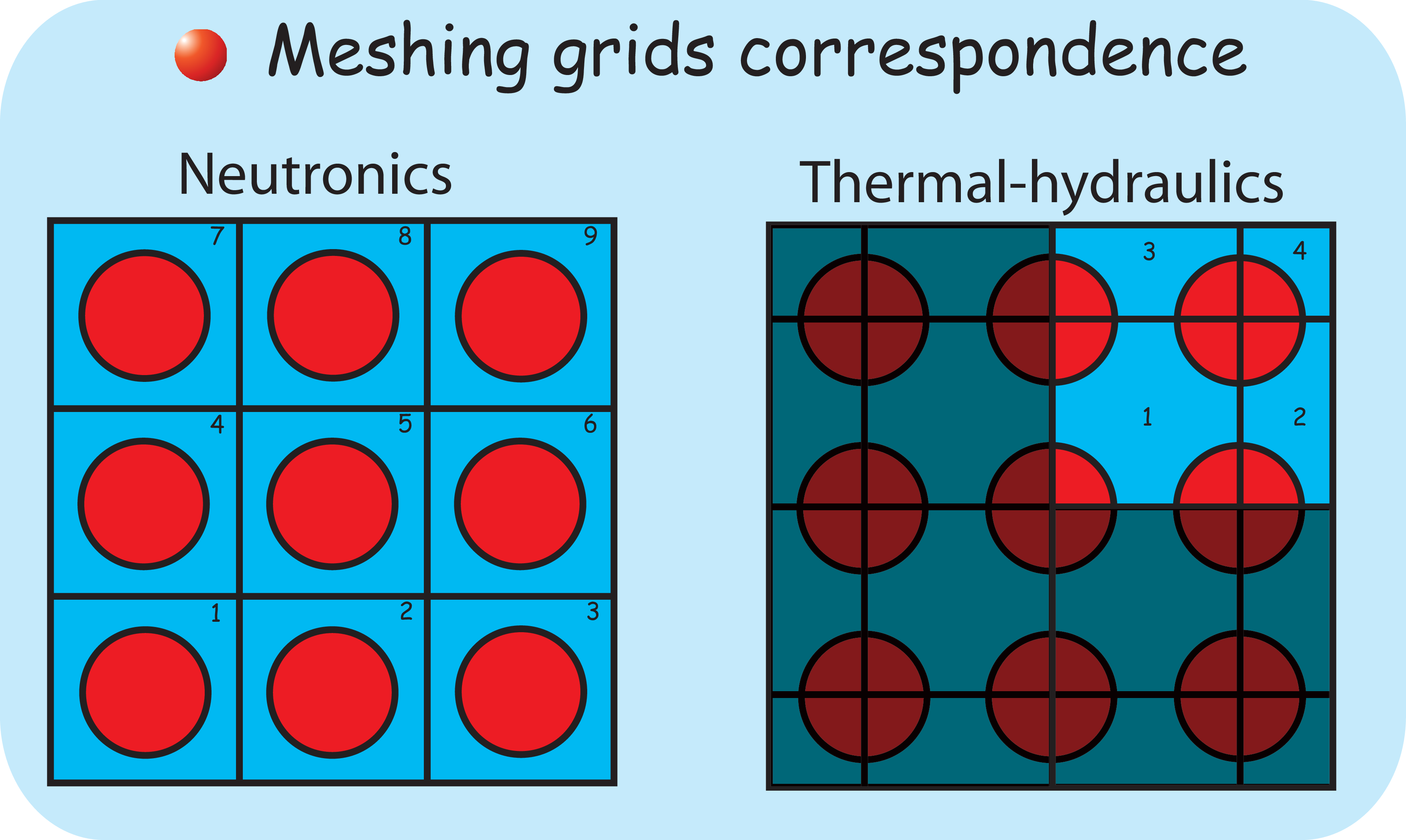
In fact two different physics disciplines are dealt with, but their solving methods have nothing in common. This is the reason why two different meshes are defined. Consequently classes manage the correspondence and the symmetrization of these meshes. Updates are done using mean values by zones (c.f. figure 9.2).
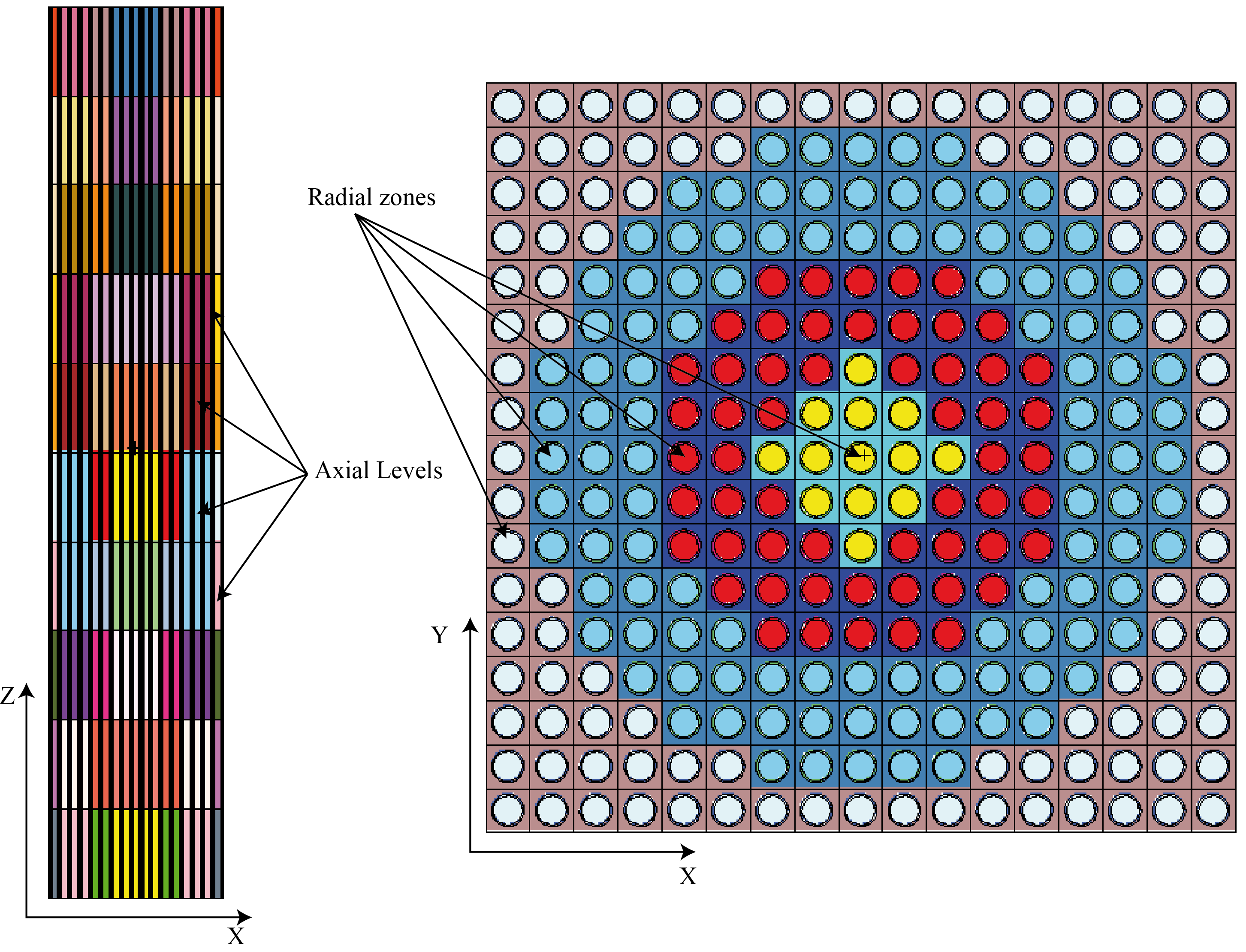
These zones are chosen by the user and are dependent on the precision required. In each radial zone and axial level, neutron flux, reaction rates, properties of materials or coolant and fuel burn-up are treated separately.
Any increase in the discretization must be carefully considered because it may use more computing resources for a marginal accuracy gain, or even, in certain circumstances, cause a loss of precision.
9.3.2 ReactorAssembly class
The ReactorAssembly class is a complete rewriting of ReactorMesh class. This class can be used in a purely neutronics way or for thermohydraulics/Thermics-neutronics coupling. As already emphasis, when COBRA_EN is involved, some restrictions are mandatory (see § 9.2).
Utilization for pure neutronics calculation
Examples are provides in RA_1ass.cxx (1 hexagonal assembly), RA_1ass_serpent.cxx (1 cuboid assembly) and RA_lattice.cxx (a cylindrical core filled by cuboid assembly).
IMPORTANT : The order of calling method in the ReactorAssembly class is not arbitrary! This is because some methods defined and/or calculate some quantities depending on previous ones. This normally has been protected (by a MURE error). But to avoid problems here are some rules (methods not mentioned there after can be called without specific order):
-
Define a ReactorAssembly object via ReactorAssembly::ReactorAssembly(double, int, int, string)
-
Define eventually plenum thickness and materials if they exist via ReactorAssembly::SetPlenum(double, Material*, Material*) and assembly duct (assembly channel) if needed via ReactorAssembly::SetAssemblyDuct(double, Material*)
-
Assign the assembly Shape to the object via ReactorAssembly::SetAssemblyShape(Shape_ptr )
-
Add all standard fuel pins that fill the whole assembly (without specify position) via
ReactorAssembly::AddFuelPin(PinCell*) -
Add specific pins at the given position via ReactorAssembly::AddFuelPin(PinCell*, int, int) or via ReactorAssembly::AddGuideTube(PinCell*, int, int) or via ReactorAssembly::AddControlRod(PinCell*, int, int)
-
...
-
and last method to be called1 must be ReactorAssembly::BuildAssemblyGeometry()
As an example, user first defines Materials and PinCell (Fuel, Guide Tubes, Control Rods, ...) he want to use. Then, he defines the shape of the assembly (either a cuboid or a hexagon):
-
Shape_ptr AssemblyShape(new Brick(S/2., S/2., H/2.)); //cuboid assembly S x S x H
or
-
Shape_ptr AssemblyShape1(new Hexagon(H/2., S)); //Hexagon assembly with edges of size S and height H.
This shape determines the type of the ReactorAssembly (Cuboid or Hexagonal) ; if, for some reasons, the assembly shape is more complex (e.g. a cuboid assembly with a hole inside that is not filled by any pins, user should provide this complex shape as well as the real cuboid (Brick class) or hexagonal (Hexagon class) of the outer bounding shape).
Then user defines a ReactorAssembly object by given the pitch of the pin lattice and the number of radial zone and axial levels
-
ReactorAssembly* RA = new ReactorAssembly(pitch,4,10); // 4 radials zones, 10 axial levels
If equal size upper and lower plenums are needed, user should call ReactorAssembly::SetPlenum(thickness, PlenumMaterial) method before any other call to a ReactorAssembly ’s method.
The shape of the assembly is passed to the ReactorAssembly object:
-
RA->SetAssemblyShape(AssemblyShape); // physical limits
And zoning is defined by given as many radial zones as it has been defined in the constructor (in this example, 3 radial zones) ; zone number range should be 0 for the most inner zone to N for the most outer. To be noticed: all lattice cell of an assembly (i.e. pins) must belong to a defined radial zone ; this implies that the last zone must include all the pins. If zones are defined via concentric virtual circle center in the middle of the assembly, the last zone radius must be at
least equal to S∕ for a cuboid assembly of side S and to 2 × S for an hexagonal assembly of side S.
-
// Automatic differentiation of zones for structurally identical elements
// (c.f. fig 9.2)
RA->AddCircleZoneRadius(2.5*pitch,0);
RA->AddCircleZoneRadius(5*pitch,1);
RA->AddCircleZoneRadius(8*pitch,2);
RA->AddCircleZoneRadius(S/sqrt(2),3);
Then, add the pins at a given position in the (x,y) lattice : the position is a position index in the lattice (with the respect to the primitive cell lattice) ; thus the (0,0) correspond to the central primitive cell, (-1,-1) to the left down adjacent cell, ... If no position is provided, the the pin fill the whole lattice (the normal way of filling normal fuel pins) ; then user can override some of the pins by adding some specific ones to a given position
-
RA->AddFuelPin(FuelPin); // the FuelPin (PinCell *) pins fill the whole assembly.
RA->AddGuideTube(GuideTube,5,2); // add a guide tube pin at (5,2) from the assembly lattice center
RA->AddGuideTube(GuideTube,0,0); // add a guide tube pin in the center of the assembly
RA->AddGuideTube(GuideTube,-5,-2);// add a guide tube pin at (-5,-2) from the assembly lattice center
...
You can add different type of fuel pin, control rods (with ReactorAssembly::AddControlRod), ...
And then build the assembly geometry (this MUST be the last method of ReactorAssembly called):
-
RA->BuildAssemblyGeometry();
Clearly, the outside cell of the assembly cannot be defined automatically and it should be defined by user himself.
For COBRA-EN coupling, the coolant around guide tubes, control rods and fuel pin cells is the same as the ones for neighbours cells (same composition, temperature, density, ...) of the same radial zone.
A more complex example is presented in RA_complex.cxx (c.f. figure 9.3) : this example shows how to define radial zones using virtual circle radii as well as specifying the zone by a lattice position.
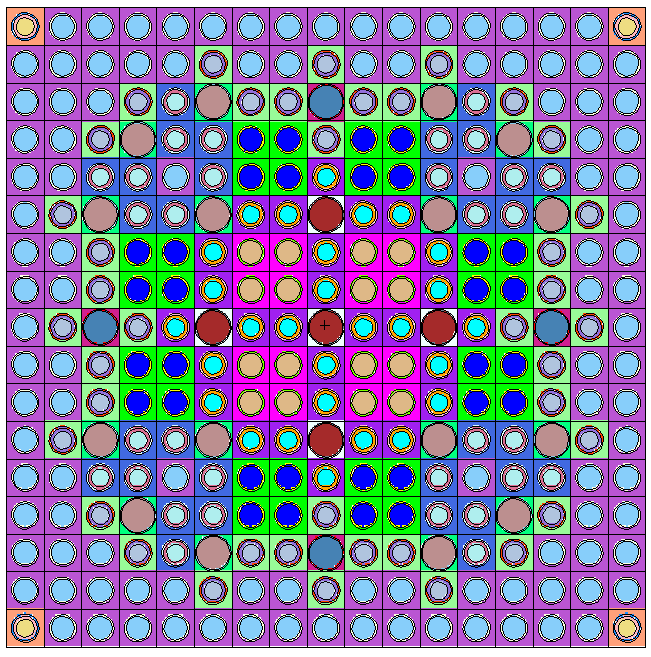
9.3.2.1 Using a ReactorAssembly to fill a core lattice
After defining a ReactorAssembly object with its fuel pins, guide tubes, plenums, ..., this assembly can be used to fill a reactor core. In order to do it, before calling the ReactorAssembly::BuildAssemblyGeometry(), one has to call the ReactorAssembly::SetUniverse() method. Then, one as to used the assembly as a lattice generator and to avoid problem of chain surface, the ReactorAssembly shape is taken as an infinite one:
-
...
ReactorAssembly* RA = new ReactorAssembly(pitch,3,3);
...
RA->SetUniverse();
RA->BuildAssemblyGeometry();
Shape_ptr InfinitAss=RA->GetInfiniteAssemblyShape();
InfinitAss->SetUniverse();
InfinitAss>>Core;
LatticeCell* LatticeGenerator=new LatticeCell(InfinitAss);
LatticeGenerator->FillLattice(RA->GetUniverse())
In this short example, the fuel core is filled with the assembly, but a more realistic filling scheme is presented in MURE/examples/RA_lattice.cxx (see Fig. 9.4).
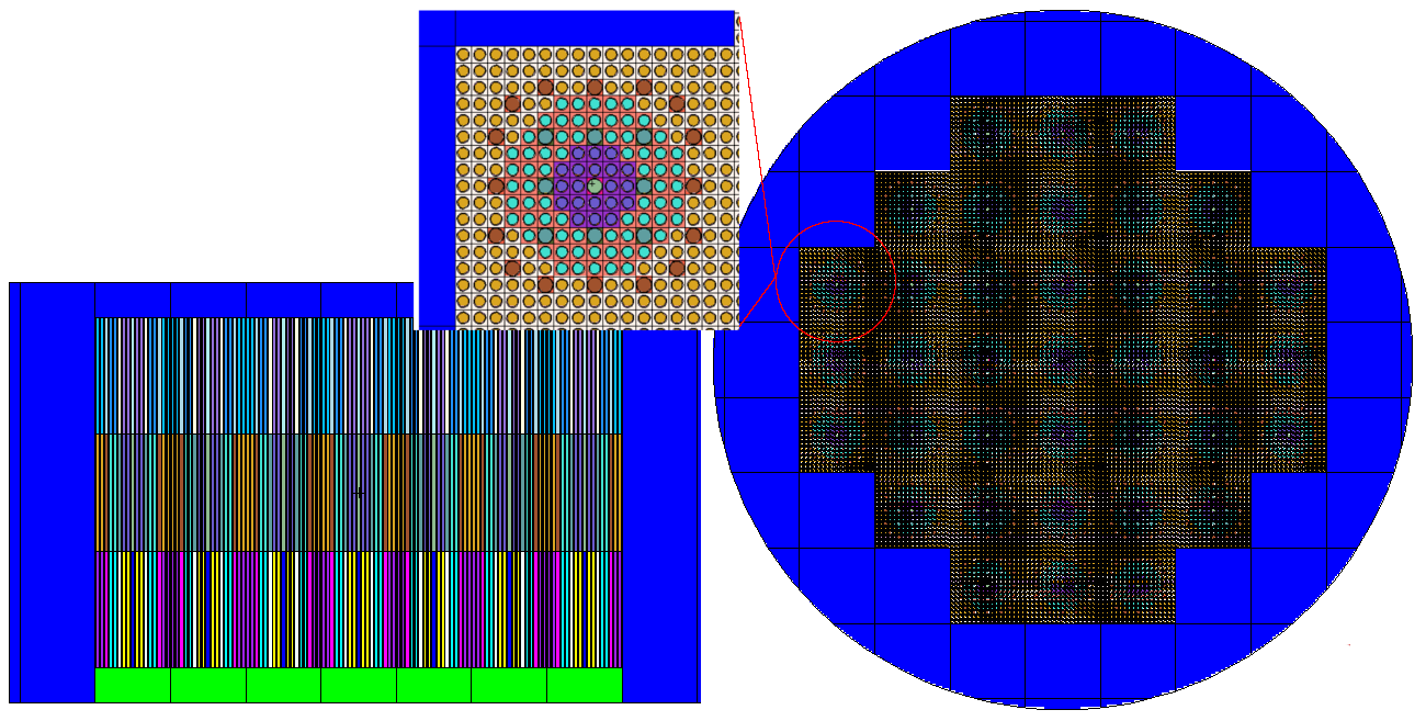
For evoltion example, see the documented example MURE/example/Evolution/RMAssembly.cxx (c.f. figure 9.5).
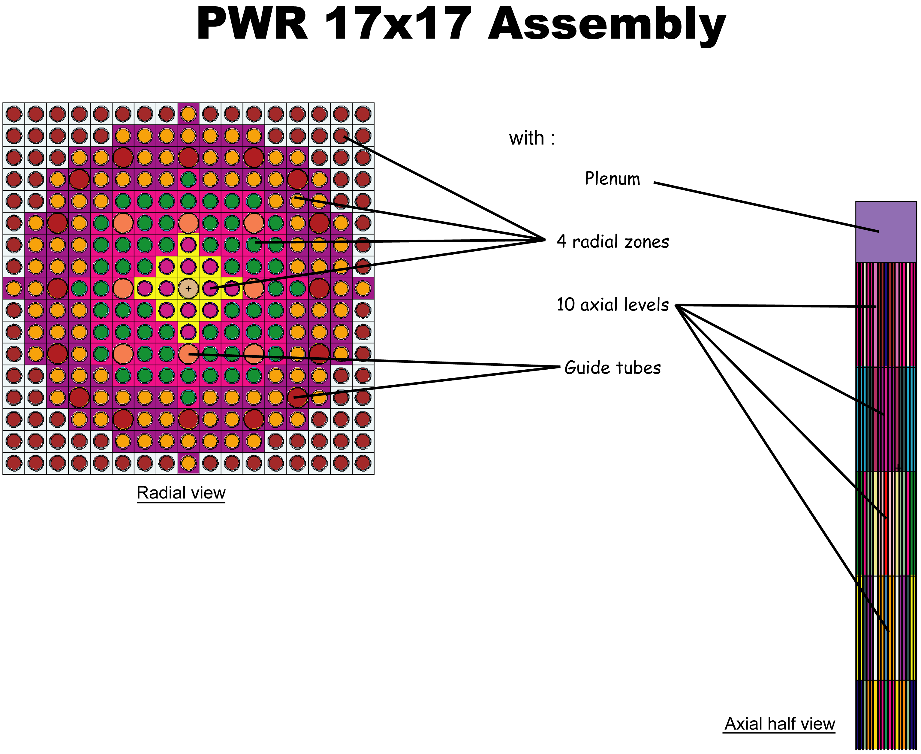
9.3.3 The COBRA_EN class : coupled neutronics/thermal-hydraulics calculations
This class manages the Oak Ridge National Laboratory code COBRA-EN (COolant Boiling in Rod Arrays). It is a sub-channel code that allows steady-state and transient analysis of the coolant in rod arrays. The simulation of flow is based on a three or four partial differential equations: conservation of mass, energy and momentum vector for the water liquid/vapor mixture (optionally a fourth equation can be added which tracks the vapor mass separately). The heat transfer model is featured by a full boiling curve, comprising the basic heat transfer regimes: single phase forced convection, sub-cooled nucleate boiling, saturated nucleate boiling, transition and film boiling. Heat conduction in the fuel and the cladding are calculated using the balance equation.
Some modifications on the source code have been done to optimize calculations on Intel Fortran Compilers (ifort) and to enlarge arrays (parameters IDSIZE in source files).
9.3.3.1 Coupling Thermo-hydraulics and neutronics
-
In the MURE input file, you must provide a gMURE->GetTemperatureMap()->SetDeltaTPrecision(Delta_T); where Delta_T is the temperature precision (in K) used to choose the closest temperature for cross-sections (this number could be big, let say arround 1500K).
-
Then, each material where temperature evolution is wanted should know it via the Material::SetTemperatureEvolution() ; this should be done for the fuel as well as for the coolant part.
-
a ReactorAssembly is built (as described above but be sure to have created real clones of evolving temperature’s materials ; for example the coolant used in fuel pins, plenums, guide tubes,... should be a different material.
-
Create a COBRA_EN object (let say this is a pointer called Channel) with the previous ReactorAssembly.
-
Set to this object the boundary conditions (inlet temperature, mass flow, exiting pressure,...), see § 9.3.3.2
-
then build and run the COBRA-EN file
-
Optionally, to achieve temperature convergence, one can loop on successive iterations between MC/thermo-hydraulics calculation.
All theses steps are exemplified in MURE/examples/Thermal/SimpleTHAssembly.cxx.
9.3.3.2 Input/Output file
The run of successive MC code and COBRA code required input files for both codes and transfer files that allow communication and cross-check of the simulation. MC file (inpXXX) is generated as usual in MURE, in the (MC) run directory. In this directory, a “TH_yyy” (where yyy is the name of the reactor assembly), input/output and transfer file for COBRA-EN are written.
-
INFILE is the COBRA-EN input file
-
OUTFILE is the COBRA-EN output file
-
Mesh_MURE_COBRA_Data.txt : are written the lattice positions for each pin in the mesh grid of neutronic code and thermalhydraulics code
-
MCNPCellsTemp.data : are written averages temperatures in each zone and level for fuels, cladding and coolant (K)
-
PowerDeposits.data : are written the local power deposits and its absolute error for a representative fuel element in each zone and level (total power released in the zone/level is normalized by the number of fuel pin in the zone - unit : W)
-
PLOTFILE is the COBRA-EN output plotfile
-
A file called yyy_MeshZoneData.txt is also created in the initial running directory: the number of fuel pins, guide tubes, special pins for each zone are quoted ; an equivalent of the mesh MCNP_Zones is also written.
Input data on operating conditions
Some precision about fluid mechanics must be given. Otherwise, default values are taken into account.
Inlet temperature (K) :
-
Channel->SetInletTemperature(560);
Average inlet mass flux (kg∕s∕m2) :
-
Channel->SetInletMassFlux(2923.72);
Inlet boron concentration (ppm) :
-
Channel->SetInletBoronConcentration(1000);
System exit pressure (MPa) :
-
Channel->SetExitPressure(15.8);
See the documented examples MURE/examples/Thermal/SimpleTHAssembly.cxx and MURE/example/Thermal/C4Assemblies.cxx (c.f. figure 9.6) and some results :
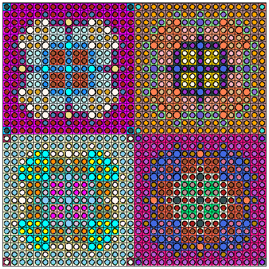
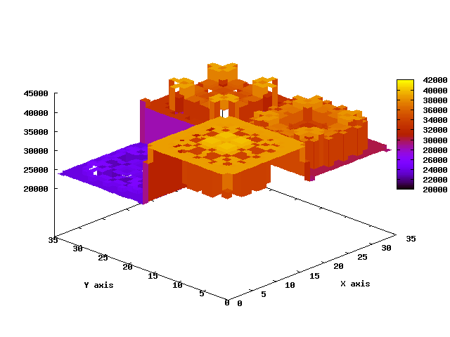 |
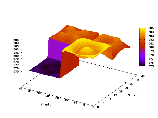 |
9.3.4 The BATH class (NOT YET TESTED IN SMURE-MURE v2.0)
This class manages temperature calculation for a coupled simulation neutronics/thermal-hydraulics with a 2D RZ precision. It is not as accurate as COBRA and must be explicitly coupled by the user but its advantages are :
-
the capability to be coupled with geometry that has already bee built
-
it is an explicit way of coupling, despite the fact it takes longer, users can completely control what is being simulated (it is not a “black box”)
-
capability to simulate a lot of coolant, cladding or fuels types: users just need to add them (thermal data and equations).
9.3.4.1 Capabilities
The code already includes data and equations necessary for simulations. It uses:
-
as fuel: uranium oxide and plutonium/uranium mixed oxide and thorium oxide (full or annular pellet)
-
as cladding: zircaloy 4 or 2 and stainless steel 316 SS
-
as coolant: light water, heavy water and sodium.
9.3.4.2 What is solved
-
heat and mass transfer:
-
steady-state forced convection in case of turbulent flows:
-
steady-state conduction inside the cladding and the fuel: Fourier law
-
radiation exchange between cladding and fuel surfaces is implemented but not used (due to a leak of precision on gas composition and evolution of the gas space dimension during burn-up): Stefan law
-
indication of pressure losses (due to acceleration, gravity and friction - loss due to peculiarity like grids are not calculated because it is considered as empirical data): acceleration is zero because the velocity is assumed constant, only gravity and friction (Darcy frictions model) are calculated
-
thermal conductivity of zircaloy and steel, data on water, sodium, UOX and MOX are from literature.
-
Nusselt dimensionless number calculation:
-
water: Dittus-Boelter equation Nu = 0.023Re0.8Pr0.4
-
sodium: Notter & Sleicher Nu = 6.3 + 0.0167Re0.85Pr0.93
-
9.3.4.3 How to add data
If thermal conductivity of new cladding is needed, one has to modify the source of ThermalCoupling class, adding flags and switching cases in ThermalCoupling::CladConduction().
To add a new coolant, equations of dimensionless number calculation are perhaps necessary and data tables must be added in thermal_data directory. As it is done for water and sodium, files containing thermal data must be created : see Water.xls in thermal_data directory.
Adding a new fuel is easier: only 2 tables of data are necessary (density and thermal conductivity : see thermal_data directory).
Contact Nicolas Capellan (capellan at lpsc.in2p3.fr) for further explanation.
9.3.4.4 Use the code
Users should create the geometry themselves. Flags will be added to indicate positions of frames and cells to the thermal-hydraulics code :
-
on materials: flag SetTemperatureEvolution() and only on fuel material SetEvolution()
-
on cells: flag(s) SetTHLevelPosition() (the first one at the bottom and then increasing height) and SetTHZonePosition() if more than one average channel is needed.
BATH is created and launched after the MCNP run.
See the documented example MURE/examples/Thermal/BATHExample.cxx.
9.3.4.5 Output data
Outputs are created in the directory called Zi_Run_j (i is the “region” and j the iteration number of coupled field).
For each level, thermal results are built together with the temperature function of distance from the center (temperature gradient inside fuel, cladding and coolant, c.f. figure 9.8).
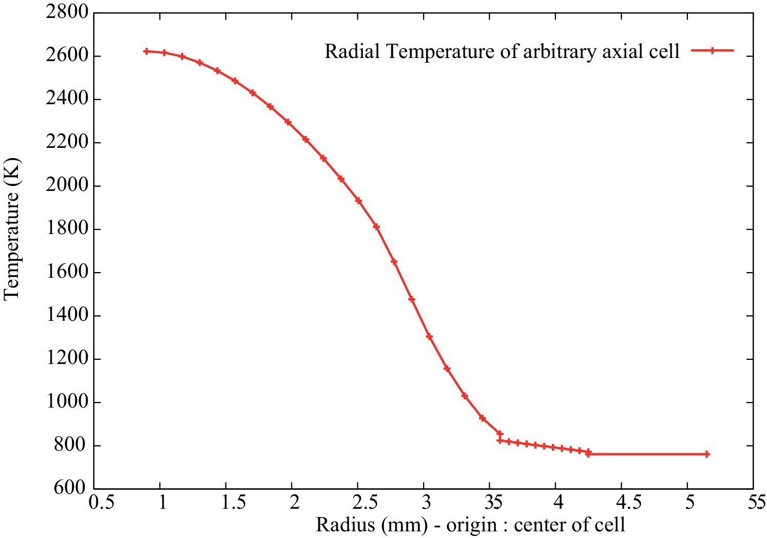
Appendix A
Basic of C++ to understand MURE
A.1 Introduction
This appendix is not a C++ tutorial ; its aim is to define roughly commonly used words inside MURE user guide and to allow users unfamiliar with C/C++ to understand examples and uses of MURE. Each main program in C++ is defined as
-
int main() //or int main(int argc, char **argv) to use argument passed to the program
{
...
}
In general, special functions, variables, ... are needed. Then, the definition of these functions known as the header files should be included:
-
#include <iostream> //standard functions for input/output on the screen (cout, cin, ...)
#include <cmath> //standard mathematical function (cos, sin, ...)
using namespace std;
#include “my_header_file.hex” //a definition made by a user
int main()
{
...
}
A.2 Class & Object
C++ is said Object Oriented. This means that the notion of variables is extended to a more complete and self consistent form: the object. The variable types are now called classes: for example, the type float of C (real in fortran) is now a class. For this class the difference between type and class is simply semantic. But you can create your own type (your own class) that regroups many other objects (or variables in C/fortran language) of different classes (different types). For example a class Point can have 2 coordinates of the class double:
-
class Point
{
public:
double X;
double Y;
};
The “public:” keyword means that one can use the objects of this class from the outside of the class. The 2 objects X and Y are called members or attributes of the class Point. To declare an object P of the class Point to be a point of coordinates (0,4), one has to
-
Point P;
P.X=0;
P.Y=4;
Moreover, a class contains methods, that is to say, specific functions that can act only on objects of this class:
-
class Point
{
public:
void Translate(double dx, double dy) {X+=dx;Y+=dy;}
double X;
double Y;
};
P can be translated of V (1,1):
-
P.Translate(1,1);
Special methods of classes are named constructors: these methods have no type and name of the class ; they are used to allocate memory and eventually initialize an object:
-
class Point
{
public:
Point(double x, double y){X=x; Y=y;}
void Translate(double dx, double dy){X+=dx;Y+=dy;}
double X;
double Y;
};
Then P can be declared as
-
Point P(0,4);
Methods (as well as functions) can be overloaded: 2 methods may have the same name but different arguments:
-
class Point
{
public:
Point(double x, double y){X=x; Y=y;}
Point(){X=0; Y=0;}
void Translate(double dx, double dy){X+=dx;Y+=dy;}
void Translate(double dV[2]){X+=dV[0];Y+=dV[1];}
double X;
double Y;
};
here the second constructor has no argument ; it is called the “default constructor” ; in this case it defines the origin point ; the second Point::Translate() method needs an array of dimension 2 as argument:
-
Point P1; //call the default constructor
Point P2(0,4); // call the “normal” constructor P2 is (0,4)
double dv[2]={1,1}; //an array of 2 doubles
P1.X=2; //set X of P1
P1.Y=2; //set Y of P1;
Point P3=P1; //P3 is (2,2)
P1.Translate(dv); //Translate P1 from (2,2)->(3,3) but P3 is still at (2,2)
P2.Translate(1,1);//Translate P2 from (0,4)->(1,5)
It is usually safe to “protect” the objects of a class from modifying them from the outside of the class without using a class method. One may succeed by using the “private:” keyword. But then one must define new methods to modify them.
-
class Point
{
public:
Point(double x, double y){X=x; Y=y;}
Point(){X=0; Y=0;}
void Translate(double dx, double dy){X+=dx;Y+=dy;}
void Translate(double dV[2]){X+=dV[0];Y+=dV[1];}
void SetX(double x){X=x;}
void SetY(double y){Y=y;}
double GetX(){return X;}
double GetY(){return Y;}
private:
double X;
double Y;
};
Then, one should not write
-
P.X=1;
cout<<”Coordinate of P(”<<P.X<<”,”<<P.Y<<”)”<<endl;
but instead, use
-
P.SetX(1);
cout<<”Coordinate of P(”<<P.GetX()<<”,”<<P.GetY()<<”)”<<endl;
Of course, this is not very useful for this simple example ; but for larger codes, it avoids bugs.
A.2.1 Header and implementation files
In the previous class Point, one has defined explicitly all methods inside the class. But when dealing with larger classes, libraries, please consider separating the class definition (.hxx files called headers) from the class implementation (.cxx files). Then, one may build libraries with implementation files whereas the header files could be included in any file using the library. For example one may rewrite the Point class header in the Point.hxx file
-
class Point
{
public:
Point(double x, double y);
Point();
void Translate(double dx, double dy);
void Translate(double dV[2]);
void SetX(double x){X=x;} // here the methods are very short,
void SetY(double y){Y=y;} // one can let then with inline definition.
double GetX(){return X;}
double GetY(){return Y;}
private:
double X;
double Y;
};
Not the “;” after the first 4 methods: it means that they will be defined somewhere else. The Point.cxx implementation file:
-
#include “Point.hxx”
Point::Point(double x, double y)
{
X=x;
Y=y;
}
Point::Point()
{
X=0;
Y=0;
}
void Point::Translate(double dx, double dy)
{
X+=dx;
Y+=dy;
}
void Point::Translate(double dV[2])
{
X+=dV[0];
Y+=dV[1];
}
Note the “Point::” ; it means that the following method belongs to the class point (“::” is the scope resolution operator).
A.3 Default arguments
In MURE, lots of parameters have default values. In general default values are assigned in methods (or function) definitions (header files) with the following syntax:
-
void TheMethod(double x=3);
This means that if one calls TheMethod(5), the value of the argument x=5, whereas a call to TheMethod() will take x=3 for this “default” argument. If one writes
-
void AnOtherMethod(double x, double y=2);
The first argument must be given and the second one (y), if it is not given, takes the value y=2. All default arguments must be defined after the explicit argument1. If one writes
-
void ThirdMethod(double x=1, double y=2, double z=1);
then a call to
-
ThirdMethod(); // means that x=1, y=2, z=1
ThirdMethod(3); // means that x=3, y=2, z=1
ThirdMethod(3,10); // means that x=3, y=10, z=1
ThirdMethod(3,10,100); // means that x=3, y=10, z=100
A.4 Pointers
We have defined objects of classes. One can define pointers on objects:
-
Point *P1=new Point; //call the default constructor
Point *P2=new Point(3,4); //call the normal constructor
P1->SetX(1); //because P1 is a pointer on a Point, one use “->” instead of the “.”
P2->Translate(1,1);
Point *P3;
P3=P1; //P3 and P1 are pointing on the same Point (1,0)
P3->Translate(1,1); // P3 and P1 point on (1,1).
Point *P;
P=new Point[3]; //P is an array of 3 Points (it points on the first)
for(int i=0; i<3; i++)
{
P[i].SetX(2*i+1); //P[i] is a Point (whereas P is a pointer)
P[i].SetY(i+1); //thus one uses a “.” and not the “->”
}
P[0].Translate(1,1); //Translate P[0] from (1,1)->(2,2)
delete P1;
delete P2;
delete [] P;
The 2 first lines allocate 2 Points (the “new” keyword). One use the “->” instead of the “.” to use a method (or a public attribute) because P1 and P2 are pointers. In the declaration of P3, no Point is allocated (no “new”) ; the “P3=P1” line means that P3 points on the same Point than P1 ; thus translating P3 will translate P1 (and vice verse). By writing “P=new Point[3]”, one allocates an array of 3 Points by calling the default constructor of Point (to declare arrays, a default constructor must exist). Each P[i] is a real Point object (not a pointer). When one use pointers, the memory is not freed by itself: one has to do it manually though a “delete”. Here one can delete P1 or P3 but not both ; in the example, P3 continues to point on the address of the P1 Point, but because the memory has been freed, this address does not correspond to anything. To delete arrays, one has to use the “[]” after the “delete” keyword.
A.5 Inheritance
One very powerful tools of classes is the inheritance mechanisms. One says that a class inherits from a mother class: all members (methods and attributes) of the mother class are known from the Daughter class. This one may have new methods and/or attributes. Following our previous example, one can define a Point3D as:
-
#include “Point.hxx”
class Point3D : public Point //here one says that Point3D is the daughter of Point
{
public:
Point3D():Point(){Z=0;}
Point3D(double x, double y, double z):Point(x,y){Z=z;}
void Translate(double dx, double dy, double dz){X+=dx;Y+=dy; Z+=dz;} //possible if the “private:” of Point
void SetZ(double z){Z=z;} //is replaced by “protected:”
double GetZ(){return Z;}
private:
double Z;
};
and one has to replace the keyword “private:” of the class Point by the keyword “protected:” in order to allow the Daughter of Point (Point3D) to modify its attributes. But from the outside of Point and Point3D, it is impossible to modify these attributes. The 2 constructors of Point3D start to call respectively the default and the normal constructor of the mother class (:Point() and :Point(x,y)).
-
Point3D P1(1,2,3); // P1 is at (1,2,3)
Point3D P2; //P2 is at (0,0,0)
P2.SetX(1);
P2.SetY(1);
P2.SetZ(1); //P2 is now at (1,1,1)
P1.Translate(1,1,1); //P2 is now at (2,2,2);
A.6 Namespace
Some classes or methods are defined in name spaces : this means that one can use a class/method with a reference to that name space : for example the use of “cout” to print a flow should be done as
-
#include <iostream>
int main()
{
...
std::cout<<”bla bla bla”<<std::endl;
...
}
But because this is sometimes quite heavy to write, one just as to use
-
#include <iostream>
using namespace std;
int main()
{
...
cout<<”bla bla bla”<<endl;
...
}
This trick is also used in MURE to choose the kind of output one need (Serpent or MCNP) ; lots of classes have the same name (e.g. the Brick class) but, because they belong to 2 different name spaces, they are doing different things. Thus one can use either MCNP::Brick or Serpent::Brick or more easily, for a “Serpent Brick”,
-
#include <iostream>
using namespace std;
using namespace Serpent;
int main()
{
...
Brick *b=new Brick(...);
...
}
Appendix B
Node tree simplification
In this appendix, more details are provided on the principle of the Node simplification to obtain more optimized MCNP input files. For example, in figure B.1 the Plane number 2 belongs to 2 Nodes and must not be destroyed after the destruction of the included node.
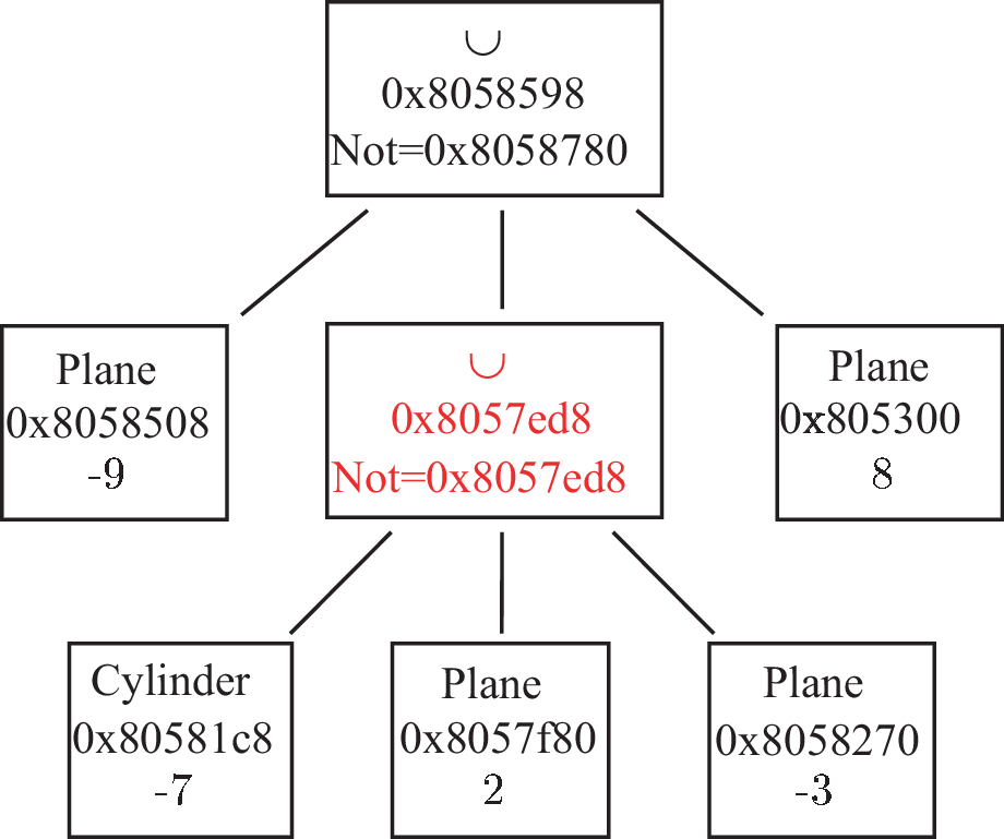
Appendix C
Stochastic volume calculation
WARNING: UP TO NOW SURFACE CALCULATIONS HAVE NOT YET BEEN IMPLEMENTED.
When using Tallies, cell volumes and/or surfaces are needed. In this package, cell volumes are calculated if possible ; when the program is not able to calculate cell volumes for a tally, we use the method ConnectorPlugin::FindMissingVolume() to extract the volume calculated by MC code itself (see note C.1). For MCNP, 2 options are available: the first one is to obtain missing volumes from the MCNP output file1 (the “o” file). Then, if all missing volume have not been found, the second option is used, that is to say a stochastic volume calculation using MCNP itself. For Serpent, only the second option is used (but of course the stochastic volume calculation use Serpent...).
The principle of the stochastic volume calculation for MCNP is to use a spherical shell neutron source geometry directed inwards containing the necessary cells filled with voids. The required volumes are calculated stochastically by MCNP from the number of particle tracks which have intersected them.
In Serpent, no transport is done, just a stochastic sampling (random points over the whole geometry) is performed.
The Serpent way of volume calculation is much faster than the MCNP way, but in general, the number of “source” particles in Serpent should be greater for a same precision (a factor 2 or 4 greater is generally enough). Nevertheless, Serpent is still faster.
The precision on volumes will depend on the “source” neutron number (that can be modified via MURE::SetVolumeNPS()) as well as the relative size of the cell/source neutron sphere. In the usual procedure, a source sphere containing the whole geometry is searched ; However, the search can sometimes fail, in which case the user is required to give the source sphere characteristics manually with the command:
-
Shape::SetVirtualSphereRadius()
and
-
Shape::SetVirtualSphereCenter()
It should be noted that it is not necessary for the whole geometry to be included in the “virtual” sphere ; only cells with unknown volumes must be inside this sphere. A volume warning message is given if the relative precision of the worst volume variance is below 0.5% ; this precision may be change with MURE::SetVolumeWarning().
C.1 Important Note
Stochastic volume calculations are used if a tally bin has a volume equal to -1. The tally bin volume is taken from the cell used in this bin. Cell volumes are determined from Shape volumes. Sometimes, we are unable to determine relatively simple Shape volumes because the Included/Disjoint method can’t return a result (e.g., a shape may be included in another one, but Shape::Included() answers 0 (i.e., not included or unknown)). For these cases it is necessary to avoid stochastic volume calculations, whereas if MC code is able to calculate the volume of such cells, we can use the method MURE::GetMCNPVolume(). For a cell without a volume (i.e. -1), if the volume has been calculated and if the cell has no universe number2, then the cell volume is set to what MC code has calculated.
To summarize, the MURE::BuildMCFile() method calls first the MURE::FindMissingVolume() method and afterward the input MCNP file is written.
NOTE: The tally bin volumes should always be provided ; thus, if a group bin or a lattice bin is used, the calculated volume related to that bin...but not to each individual cell composing the bin. Therefore, the individual cell volume remains unknown.
Appendix D
Back-Stage processes: everything you always wanted to know about MURE* (*But were afraid to ask)
D.1 Steady-state power: Tally Normalization
MCNP provides raw tallies normalized by source neutron ; we have, for the sake of simplicity, choose the same normalization method in Serpent.
For reactor applications, in order to simulate a constant reactor power1, one must normalize all tallies by the equivalent number of neutrons per second for a user-given power value. This normalization factor will change as the isotopic composition of the material evolves with time and therefore needs to be calculated at the lowest level of time discretization, i.e., at every sub-step (CRAM/RK ones), and, a fortiori, also every time neutron transport is performed.
-
Constant power P is defined by the user once and for all throughout the evolution using the gMURE->SetPower() function . This value is translated into the number of fissions per second.
-
At every MC step, flux ϕ and average reactions cross-sections σiare read from MC output for every nucleus in every cell. Isotopic proportions are read from the initial user-defined composition and for all subsequent steps these values are solved according to their Bateman equations.
-
At every CRAM/RK sub-step average cross-sections σi, read in the prior MC step, have (so far) been kept constant. New values for the isotopic proportions Ni+1 are solved for using former values of other parameters. P is constant by definition : a new value of the tally normalization factor is therefore calculated in order to keep P constant.
D.1.1 Energy Released from MURE fissions
The energy released per fission is around 200 MeV, but the exact value varies by +/- 5% and varies primarily with the mass of the fissile isotope.
By default MURE assumes that the energy released from fission for each fissionable isotope is different. For several common fissile isotopes, the fission energy values are taken from: W.H. Walerk, “Mass balance estimate of energy per fission in reactors AECL-3109, 1968”. For all other fissionable isotopes, fitted values are used. The linear fit (as a function of mass) is made for the common isotopes [232Th - 241Pu] and extrapolated to the uncommon ones.
For example (see [39]), in the case of 235U, the energy released by fission Q is given in Table D.1.
|
|
|
| Fission Product kinetic energy | 166.2 ± 1.3 MeV |
|
|
|
| Prompt fission γ | 8.0 ± 0.8 MeV |
|
|
|
| Delayed (after β decays) γ | 7.2 ± 1.1 MeV |
|
|
|
| β decays | 7.0 ± 0.3 MeV |
|
|
|
| Neutron kinetic energy | 4.8 ± 0.1 MeV |
|
|
|
| (n,γ) capture(6 MeV × 1.42 neutrons) | 8.5 MeV |
|
|
|
| Energy released Q | 201.7 ± 0.6 MeV |
|
|
|
In MURE, the default value is Q235U = 201.7 MeV. The energy of neutrinos (in this case, 9.6 MeV), is not taken into account.
If a user wishes to use specific values, 2 methods are available. The first one, MURE::SetAllFissionEnergies() allows to give a common constant value to each fissionable isotopes (default=200 MeV) ; the second method, MURE::SetFissionReleasedFile() allows user to give a file with the required value for some (or all) fissionable isotopes. Each line of the file is
-
Z A Qvalue
where Z and A are the proton and nucleon numbers and Qvalue is the energy released by fission (in eV). When using this method, the Q values are taken as explained above (using the linear fit) except for the isotopes specified in this file.
NOTE: MURE::SetAllFissionEnergies() and MURE::SetFissionReleasedFile() must be called BEFORE any Material declaration to be taken into account.
The fact that MURE takes into account different fission energy released values, means that there will be slight differences in the way the normalization factor is calculated, and therefore slight difference in inventory when the fissile nucleus changes as a function of time when compared with the old method.
D.1.2 How the normalization factor is calculated
The total power delivered by the total number of fissions in a given instant (in MC raw units) is given by the double sum shown hereafter :
where the subscript i refers to the nucleus considered whereas j refers to the cell considered. The sum is to be carried out over all cells and all nuclei belonging to each cell’s material.
PMC can be thought of as the power delivered per source particle transported in the global geometry in question : If ϕj is in standard MC cell tally output units (particles per unit surface per source particle) then PMC will be also normalized per source particle.
-
Nijis the number of nuclei i present in cell j.
-
σij is the average fission cross-section of nucleus i in cell j.
-
ϕj is MC’s neutron flux track-length estimation for cell j.
-
ξ is the average energy delivered in one fission (∼200 MeV).
Therefore, the scaling factor α, by which tallies will be normalized and which has to be taken into account in order to simulate a constant burn-up at the desired power Puser (if Puseris provided in watts and ξ in eV) is written :
D.1.3 An alternative approach
For a critical system, if one multiplies the desired power in fissions per second times the average number ν of neutrons emitted per fission, one obtains the amount of existing neutrons in the geometry at a given instant. This can be thought of as the intensity of the neutron source needed to achieve this desired power. This value, in neutrons per second, should be equivalent to the value of α calculated in the previous paragraph. If the system is critical (Keff = 1) this number is constant during a time interval small enough so that the amount of fissile material remains unchanged in a first approximation. If the system is critical and Puser is in unit Watt and ξ in unit Electron-Volt, then:
For our problem example, the first method gives a value of alpha of roughly 8.28010+12 whereas the second method gives a value of 8.12410+12 with νtaken at 2.599. The two values are therefore comparable within less than 2 percent.
This normalization can be activated by setting
-
gMURE->GetEvolutionSolver()->SetPowerNormalizationFactorNuOverKeff();
in the input. MURE will add appropriate global tallies to calculate the systems ν.
Bibliography
[1] O. Méplan, A. Nuttin, O. Laulan, S. David, F. Michel-Sendis, and J. Wilson. MURE: MCNP Utility for Reactor Evolution – Description of the methods, first applications and results. In European Nuclear Society, editor, ENC 2005-European Nuclear Conference. Nuclear Power for the XXIst Century: From basic research to high-tech industry, pages 1–7, 2005.
[2] F. Michel-Sendis, O. Méplan, S. David, A. Nuttin, A. Bidaud, J. N. Wilson, and O. Laulan. Plutonium incineration and uranium 233 production in thorium fueled light water reactors. In GLOBAL 2005: International Conference on Nuclear Energy Systems for Future Generation and Global Sustainability, page 132, Tsukuba, Japan, October 2005. Tsukuba National Laboratory For High Energy Physics.
[3] X-5 Monte Carlo Team. MCNP – A General Monte CarloN-Particle Transport Code, Version 5. Technical report, Los Alamos National Laboratory, LA-UR-03-1987, April 2003.
[4] Jaakko Leppänen, Maria Pusa, Tuomas Viitanen, Ville Valtavirta, and Toni Kaltiaisenaho. The Serpent Monte Carlo code: Status, development and applications in 2013. Annals of Nuclear Energy, 82:142–150, August 2015.
[5] M. Aufiero, A. Cammi, C. Fiorina, J. Leppänen, L. Luzzi, and M. E. Ricotti. An extended version of the SERPENT-2 code to investigate fuel burn-up and core material evolution of the Molten Salt Fast Reactor. Journal of Nuclear Materials, 441:473–486, 2013.
[6] J. S. Hendricks, G. W. McKinney, H. R. Trellue, J. W. Durkee, T. L. Roberts, H. W. Egdorf, J. P. Finch, M. L. Fensin, M. R. James, D. B. Pelowitz, and L. S. Waters. MCNPX version 2.6.A . Technical report, Los Alamos National Laboratory report LA-UR-05-8225, 2005.
[7] D. I. Poston and H. R. Trellue. User‘s manual, version 2.0 for Monteburns, version 5B, Los Alamos National Laboratory report LA-UR-99-4999, 1999.
[8] L. M. Petrie, W. C. Jordon, and A. L. Edwards. SCALE: a modular code system for performing standardized computer analyses for licensing evaluation. version 5.1 – Volume 1-3, ORNL/TM-2005/39, 2006.
[9] R. S. Babcock, D. E. Wessol, C. A. Wemple, and S. C. Mason. The MOCUP Interface: A Coupled Monte Carlo/Depletion System. In Topical Meeting on Advances in Reactor Physics, Knoxville, TN, volume III, page 368, April 1994.
[10] J. Cetnar, W. Gudowski, and J. Wallenius. MCB: A continuous energy Monte Carlo Burnup simulation code. Technical report, Actinide and Fission Product Partitioning and Transmutation, OCDE/NEA, 1999.
[11] W. Haeck and B. Verboomen. VESTA, An Optimum Approach to Monte Carlo Burnup. Nuclear Science and Engineering, 156(2):180–196, June 2007.
[12] J. Miss, O. Jacquet, F. Bernard, B. Forestier, W. Haeck, and Y. Richet. First validation of the new continuous energy version of the MORET5 Monte Carlo code. In International Conference on the Physics of Reactors, PHYSOR 2008, 2008.
[13] Emeric Brun, Eric Dumonteil, and Fausto Malvagi. Systematic uncertainty due to dtatistics in Monte Carlo burnup codes: Application to a simple benchmark with TRIPOLI-4-D. Progress in Nuclear Science and Technology, 2(0):879–885, October 2011.
[14] Jason Chao. COBRA-3C/RERTR - A Thermal-Hydraulic Subchannel Code with Low Pressure Capabilities. Technical report, Science Applications, Inc., December 1980.
[15] D. Basile, R. Chierici, M. Beghi, E. Salina, and E. Brega. COBRA-EN, an Updated Version of the COBRA-3C/MIT Code for Thermal-Hydraulic Transient Analysis of Light Water Reactor Fuel Assemblies and Cores. Technical report, OECD/NEA, 1999.
[16] R. E. MacFarlane and D. W. Muir. The NJOY Nuclear Data Processing System Version 91. Technical report, Los Alamos National Laboratory report LA-12740-M, 1994.
[17] J. R. Parrington, H. D. Knox, S. L. Breneman, E. M. Baum, and F. Feiner. Chart of the nuclides. fifteenth edition, revised to 1996. Technical report, Knolls Atomic Power Lab., Schenectady, NY (United States), 1996.
[18] Richard B. Firestone, Coral M. Baglin, and S. Y. Frank Chu, editors. Table of isotopes. Wiley, New York, 1999.
[19] Mark A. Kellett, Olivier Bersillon, and R. W. Mills. The JEFF-3.1/-3.1.1 radioactive decay data and fission yields sub-libraries. Technical Report NEA 6287, Nuclear Energy Agency, 2009.
[20] Gaël Guennebaud, Benoît Jacob, et al. Eigen v3. http://eigen.tuxfamily.org, 2010.
[21] Niels Lohmann. JSON for Modern C++. https://github.com/nlohmann/json, 2013-2021.
[22] Patrick Boettcher. JSON schema validator for JSON for Modern C++. https://github.com/pboettch/json-schema-validator, 2020.
[23] American National Standard. Neutron and gamma-ray flux-to-dose rate factors, ANSI/ANS–6.1.1, 1977.
[24] D. E. Cullen. PREPRO 2019: ENDF/B Pre-Processing Codes. IAEA-NDS-39, Rev. 19.
[25] A. J. Koning, D. Rochman, S. van der Marck, J. Kopecky, J. Ch. Sublet, S. Pomp, H. Sjostrand, R. Forrest, E. Bauge, H. Henriksson, O. Cabellos, S. Goriely, J. Leppanen, H. Leeb, A. Plompen, and R. Mills. TENDL-2014: TALYS-based evaluated nuclear data library.
[26] R. E. MacFarlane. The NJOY Nuclear Data Processing System, Version 2016. LA-UR-17-20093.
[27] M. Oettingen, C. Döderlein, E. D’Agata, K. Tuček, and J. Cetnar. Comparison of MCB and FISPACT burn-up performances using the HELIOS experiment technical specifications. Nuclear Engineering and Design, 242:399–412, January 2012.
[28] M. J. Bell. ORIGEN: The ORNL Isotope Generation and Depletion Code. ORNL-4628. Oak Ridge National Laboratory, 1973.
[29] A. G. Croff. ORIGEN2: A versatile computer code for calculating the nuclide compositions and characteristics of nuclear materials. Nucl. Technol., 62:335–352, 1983.
[30] William Press. Numerical recipes in C : the art of scientific computing. Cambridge University Press, Cambridge Cambridgeshire New York, 1992.
[31] Maria Pusa and Jaakko LeppÀnen. Computing the Matrix Exponential in Burnup Calculations. Nuclear Science and Engineering, 164(2):140–150, February 2010.
[32] Maria Pusa. Numerical methods for nuclear fuel burnup calculations. Aalto University, 2013.
[33] Maria Pusa. Higher-Order Chebyshev Rational Approximation Method and Application to Burnup Equations. Nuclear Science and Engineering, 182(3):297–318, March 2016.
[34] Maarten Becker. Code and Data Enhancements of the MURE C++ Environment for Monte-Carlo Simulation and Depletion. atw - International Journal for Nuclear Power, 65(6/7):337–340, 2020.
[35] Timothy A. Davis. Algorithm 832: UMFPACK V4.3—an unsymmetric-pattern multifrontal method. 30(2):196–199.
[36] E. F. Shores. Data updates for the SOURCES-4A computer code. Nuclear Instruments and Methods in Physics Research Section B: Beam Interactions with Materials and Atoms, 179(1):78–82, June 2001.
[37] James F. Ziegler and Jochen P. Biersack. The Stopping and Range of Ions in Matter, 1985.
[38] W. B. Wilson, M. Bozoian, and R. T. Perry. Calculated α-induced thick target neutron yields and spectra, with comparison to measured data. Technical report, 1988.
[39] M. F. James. Energy released in fission. Journal of Nuclear Energy, 23(9):517–536, November 1969.

